When data collected has a geographic dimension it may be interesting to visualize it on a map by using the R library map.
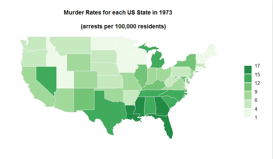
In this example, we visualize the murder rates by US state back in 1973. That's almost 45 years ago!
The following code does just that. The R code in the snippet bellow explains this in just a few lines where each step is well commented
} You can even copy paste the code in Rstudio and there are also the libraries to import. Try to understand the code (by going through the lines and comments) before you run it. And here is the result This is one more example of how great R programming language is for making data visualizations of this type. Stay tuned for more ;-)
//import libraries
library(maps)
library(WDI)
library(RColorBrewer)
x = map("state",plot=FALSE)
for(i in 1:length(rownames(USArrests))) {
for(j in 1:length(x$names)) {
if(grepl(rownames(USArrests)[i],x$names[j],ignore.case=T))
x$measure[j] = as.double(USArrests$Murder[i])
}
}
colors = brewer.pal(7,"Reds")
sd = data.frame(col=colors,
values=seq(min(x$measure[!is.na(x$measure)]),
max(x$measure[!is.na(x$measure)])*1.0001,
length.out=7))
breaks = sd$values
matchcol = function(y) {
as.character(sd$col[findInterval(y,sd$values)])
layout(matrix(data=c(2,1), nrow=1, ncol=2),
widths=c(8,1), heights=c(8,1))
// Color Scale below
par(mar = c(20,1,20,7),oma=c(0.2,0.2,0.2,0.2),mex=0.5)
image(x=1, y=0:length(breaks),z=t(matrix(breaks))*1.001,
col=colors[1:length(breaks)-1],axes=FALSE,breaks=breaks,
xlab="", ylab="", xaxt="n")
axis(4,at=0:(length(breaks)-1),
labels=round(breaks),col="white",las=1)
abline(h=c(1:length(breaks)),col="white",lwd=2,xpd=F)
// Draw the Map
map("state", boundary = FALSE,col=matchcol(x$measure),
fill=TRUE,lty="blank")
map("state", col="white",add = TRUE)
title("Murder Rates by US State in 1973 \n
(arrests per 100,000 residents)", line=2)