How Chaos Theory applies in fractals, with tutorial and source code
Just recently @drwatson mentioned chaos theory in the comments of a fractal post, and in so doing, inspired this post. In short, Chaos Theory is about very small changes that have great and unpredictable results in a larger scale. The pioneer of Chaos Theory was Edward Lorenz, a meteorologist, who explained that the formation and paths of weather phenomena (like a hurricane) may depend on very subtle conditions, like the flap of a butterfly’s wings in China causing a tornado in Brazil! While this is an over-dramatization that cannot be verified, it illustrates the concept very well.
Also, things will get a bit ... fractally technical, so draw a deep breath before continuing!
All the fractals used in this post were created in JWildFire, a free-to-use open-source application. The definition of each fractal in XML is available in Pastebin to keep this post clean & tidy. You can paste those into JWildFire and try the same modifications I detail below to see the results yourself.
Fractal Curve
(XML source in pastebin.com)
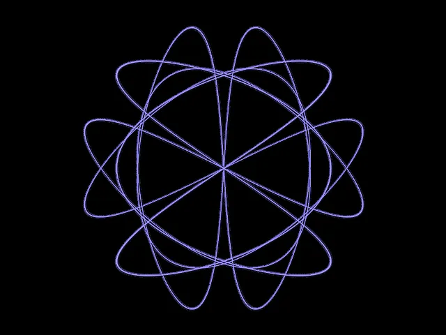
We will start with something easy, and build on it to see the changes one by one. I am using point symmetry, which means that the final image is symmetrical with respect to the origin (the center). The variation “lissajuss” creates a curve according to the parameters entered. For the set of parameters (3, 2, 0, 0, 0) it draws this curve:
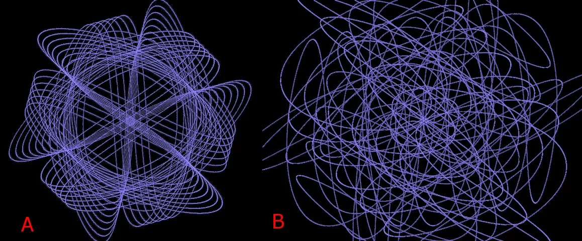
When the 3rd parameter is increased by just 0.01 we get the following fractal; as you can see in pic A, it retains the original geometry but is very different. Now, lets increase all parameters by 0.05, except the 5th one; the new input set is (3.05, 2.05, 1.05, 1.05, 0) and it draws the complex curve shown in pic B, which bears no resemblance to the original curve:
To complete the first demo, the 5th parameter is increased by just 0,05 too:
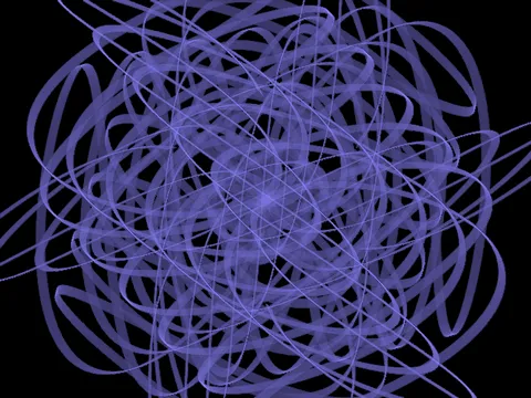
Now that the effect of these small tweaks is evident, let’s add some extra variations, to get a more impressive fractal, something that looks like fine line-art. I deliberately used a monochrome palette for this series, as the objective here is to showcase the importance of small changes.
Fractal Grid
(XML source in pastebin.com)
Now, let’s try something more … swirly! First, a combination of 2x “linear3d” and 1x “cpow3” variations gives the simple grid of the screenshot below:
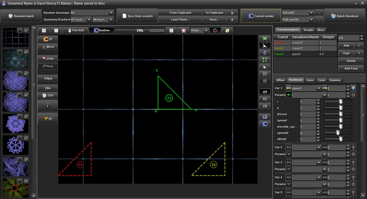
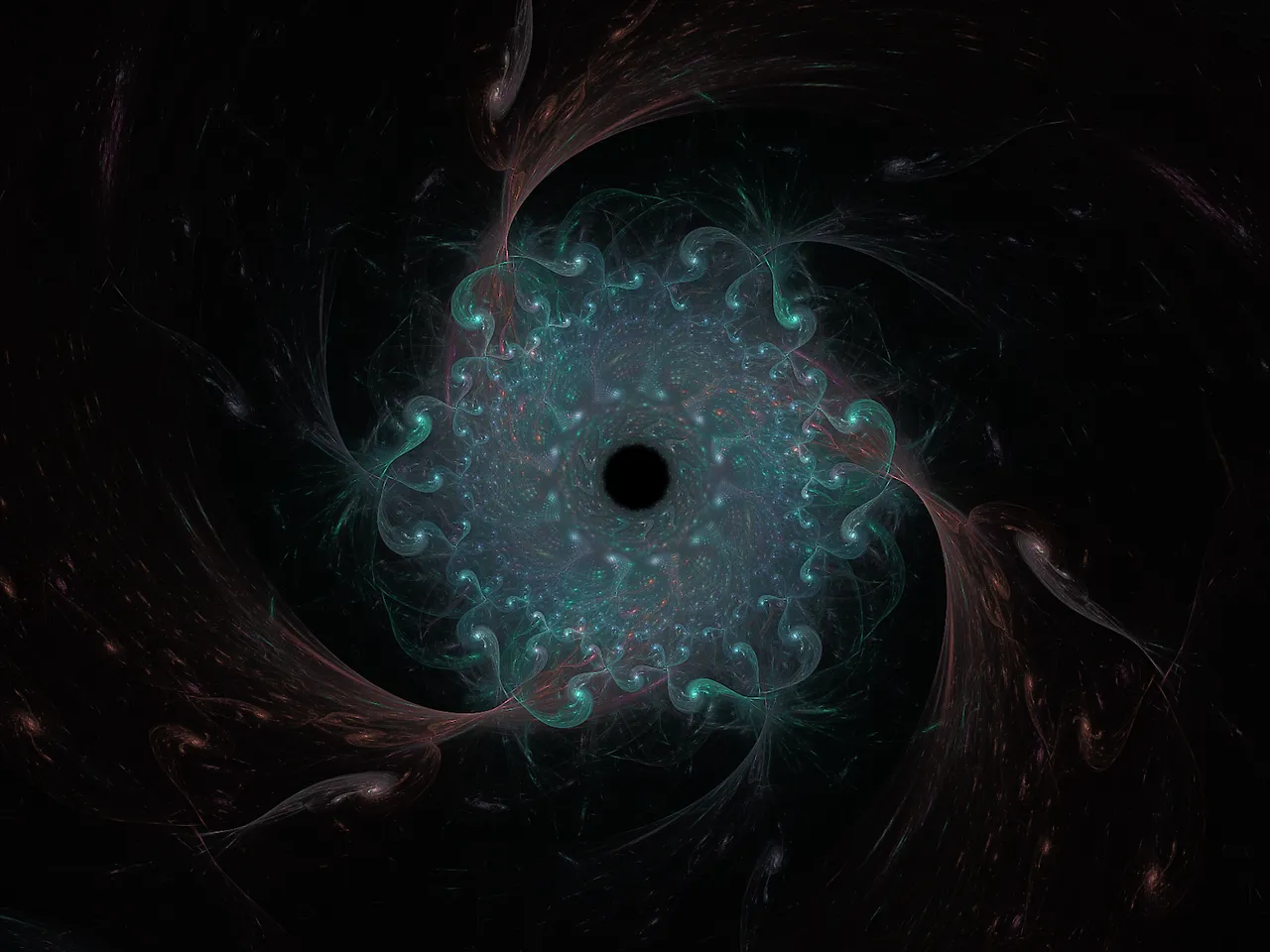
The “cpow3” variation uses several variables, but we will change just one: variable a is increased by 0.01 in the 1st picture and by 0.1 in the second. When these minute changes go through hundreds & hundreds of iterations of the other variations and each time are fed back to “cpow3”, ultimately, they scale up and produce something completely different:

As you can see in the pics above, fractions like 0.01 are fed again & again into the formulas, are skewed and twisted into new shapes and patterns and new detail emerges where previously there were just straight lines.
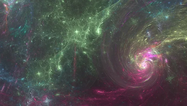
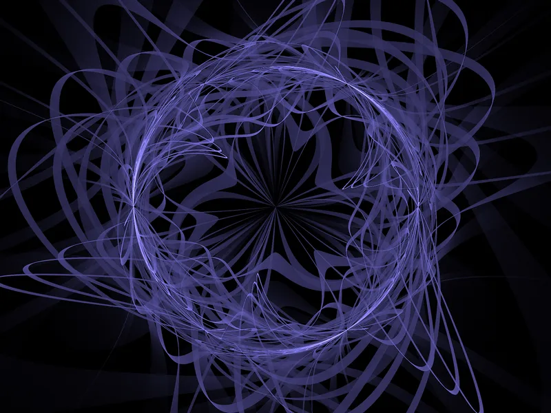
Now, for some eye-candy, let’s add some color shifts and a “julia3d” variation, as final. In JWildFire, final variations are not fed-back and re-iterated as the normal variations, it is like finalizing the fractal transformation. And in the end, another gradient and a “mobius” final variation instead of “julia3d” take us on a flight into the nebulas of distant space...
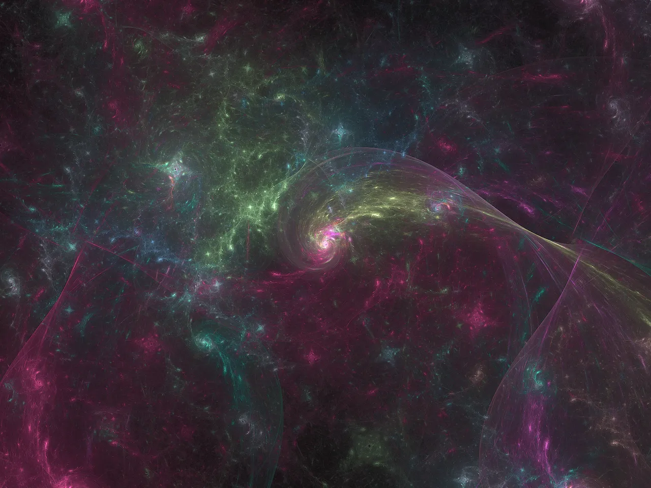
(right-click -> "open in new tab" for full size - XML source of the nebula in pastebin.com)
That was just a brief outline of how things work in JWildFire, and how modifying some parameters even by a small amount may result in drastically different fractals. Did you enjoy this as much as I did, or am I just an obsessed nerd mesmerized by decimal numbers??