If you have ever experienced randomly finding a beautiful stone laying on the ground, you may be able to understand the allure that entices rockhounds to pursue their endless quest. The determined search often ends with a disappointing and lackluster collection of dull stones gathered as an insurance policy against coming out empty-handed.

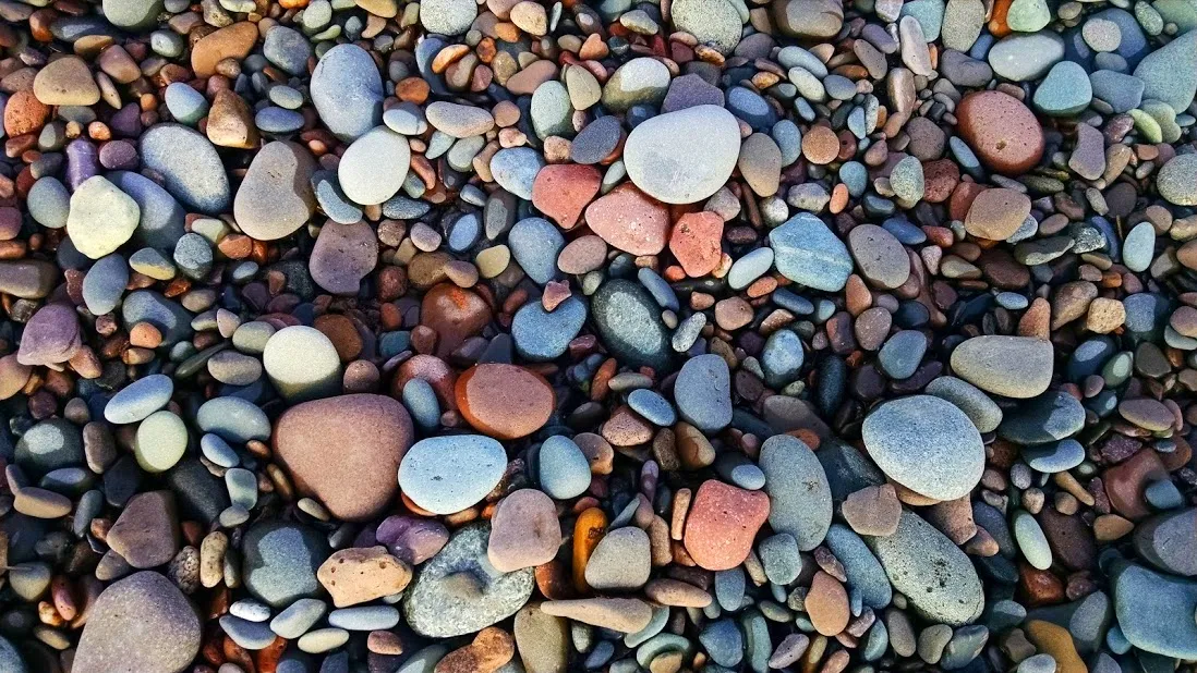^{Though some might consider these dull, any wave-washed rock has a certain appeal.}

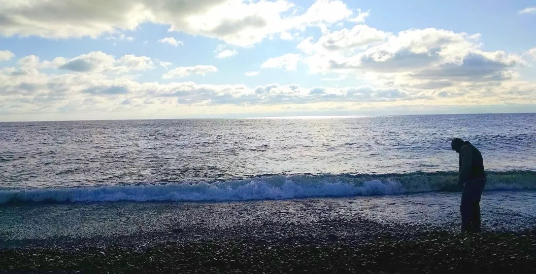
On occasion, the odds are reversed. A glimmering reflection might catch the eye of a meditative pacer as lapping waves on a rocky beach set time. Or maybe a walk down the creek in a local park reveals a unique geologic treat hiding amongst otherwise nondescript specimens. These chance occurrences are enough to fuel the continued efforts of a dedicated 'hounder', as the only point of certainty is this: You will never find them unless you look.

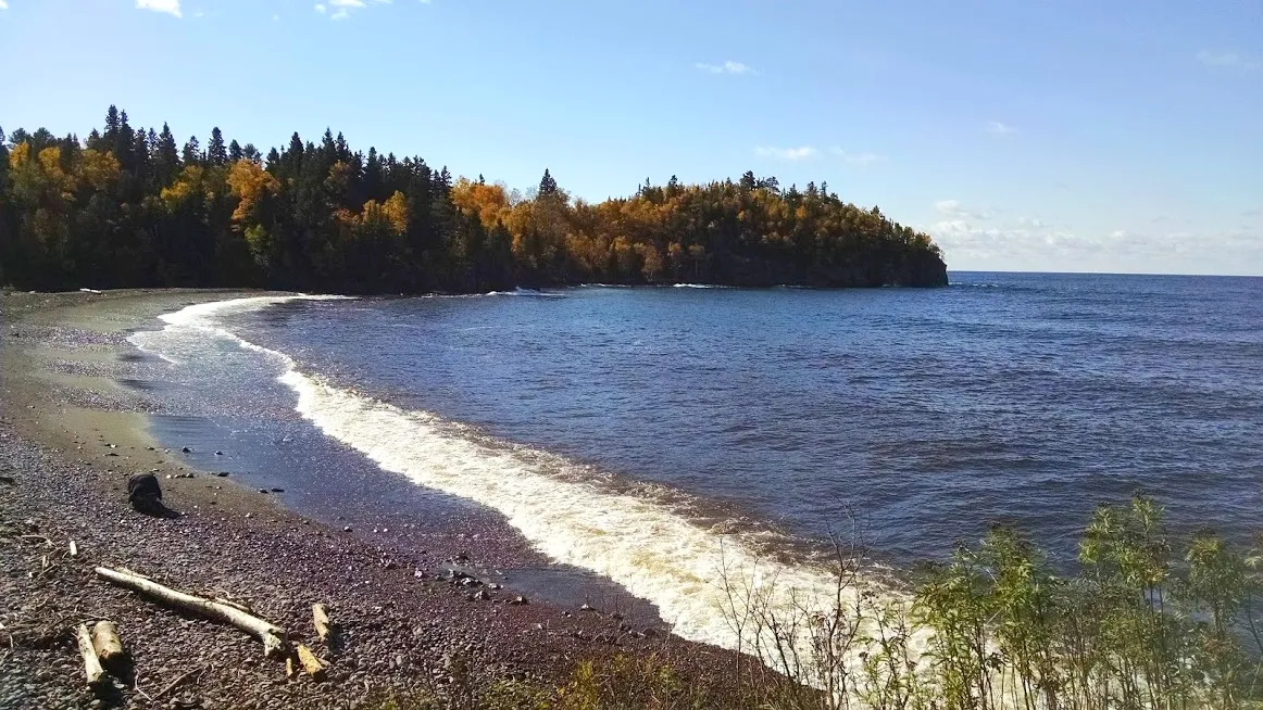
^{Few things are more calming than scanning the endless sea of a rocky beach.}

While this principle applies broadly, in this instance we are revisiting a special type of gemstone that I have discussed previously: Lake Superior Agates. In this article we learned how and where they form, admired their stunning beauty, and established a rough idea of their spatial distribution based on the extents of the last glaciation(s). In this article, we will examine how spatial data can be used to identify the best areas to hunt for these incredible stones!

^{Even when the target rock is not found, the places where you search are often a treat in themselves.}

Care To Join?

The software and the data referenced in this article are freely available and can be installed on practically any device. If you want to follow along and try doing this yourself, download the incredible open-source program QGIS HERE. A fresh new version (3.0) was recently released, so now is a great time to learn the wonders of GIS! Personally, I am still using an older version of QGIS (2.6) to maintain compatibility with some plugins that I require.

^{Source under CC-BY-SA - The latest version of QGIS is powerful, intuitive, and elegant!}

Digging Up Data

There is a wealth of geologic spatial data to consider that might help with finding agates. An initial thought was to look at bedrock geology and identify the distribution of the basalt flows where the agates originate. This will work in areas where bedrock is exposed at the surface, but most of the bedrock in the Upper Midwest is buried by more than 100 feet of glacial material (See Figure 1 in the Deposit Thickness section below). In addition, the bedrock would still need to be mined to expose agates. For now we will focus on unconsolidated material that the glaciers churned up and left behind.

Surficial Geology

Geologic material that has yet to be consolidated into rock (lithified) is known as 'surficial' geology. It is sometimes referred to as 'Quaternary' geology in reference to the most recent period of geologic time. Multiple glaciations left material throughout upper North America during the Quaternary.

^{Source by sumanamul15 under CC0 - Continental glaciers act as a massive bulldozer, stirring up rock and grinding it into clay.}

Unconsolidated material is generally differentiated by the grain size and sorting of the sediment, an attribute related to the depositional environment. We'll have to understand the geologic terms used to describe surficial geology in order to best prioritize the data for finding agates. These terms and names can vary greatly between data sets and authors, making the task of deciphering the meaning and correlating units a challenging geospatial puzzle...Settle in - this post will be fairly comprehensive!

National Scale

For the purposes of this article, I have chosen to work with data from a national level. The US Geological Survey published a map and data set of the surficial geology of the United States at a 1:5,000,000 scale in 2009. This data covers most of the potential range of Lake Superior Agates (omitting Canada).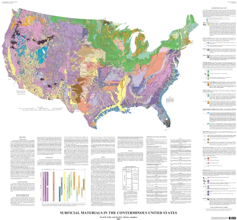

^{Source [a] - USGS Publication from 2009 showing the surficial geology of the mainland US.}

While the map is useful for reference, a digitized version of the data allows for a more customized data analysis. The GIS data set can be downloaded as a Shapefile or as a Geodatabase. While the geodatabase is smaller in size, this format is a proprietary file type that can only be read by ArcGIS (by ESRI). Many University students have access to this software at no cost, but in this article we will use Shapefiles as they are easy to work with in either software suite.

Loading Shapefiles

The US surficial Shapefile based on the above publication is 112 MB in size and can be downloaded HERE. Once downloaded, the zipped folder must be unpacked using native decompression software before it can be opened with QGIS. The unzipped folder contains 24 files, including three shapefiles (also known as vector files).

To add the Shapefiles in QGIS, go to Layer -> Add Layer -> Add Vector Layer and click browse to change the source to the unzipped folder. Sort by type and find the three files with the file extension .shp - Contacts, State_Lines, and Surficial_materials. 'Contacts' is a line file tracing the surficial polygons that will not need to be loaded for this analysis. The other two layers, however, will both be useful to load. The 'State_lines' layer outlines state boundaries, and the 'Surficial_materials' layer contains polygons encompassing unconsolidated material.

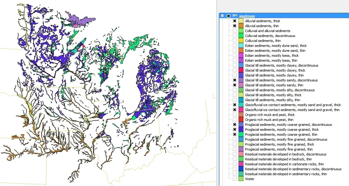
^{1:5,000,000 Surficial Geology Shapefile for the continental US. All features are colored the same by default upon initial load.}

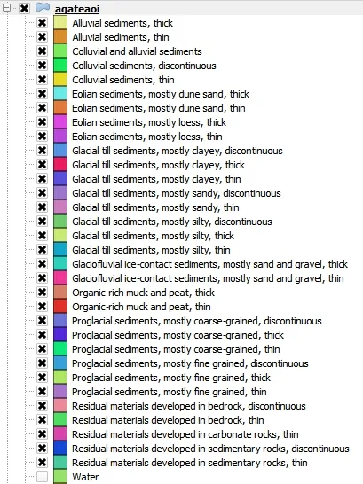
Unit Name

To differentiate the monochrome units and get a view that is similar to the USGS published map, we need to adjust the style of the layer. Right-click the 'Surficial_materials' layer in the Layers Menu and select Properties to bring up the style options. Toggle the first option from Single Symbol to Categorized and select UNIT_NAME as the Column. Now we simply Classify the data to assign random colors to each unit. Here is the result: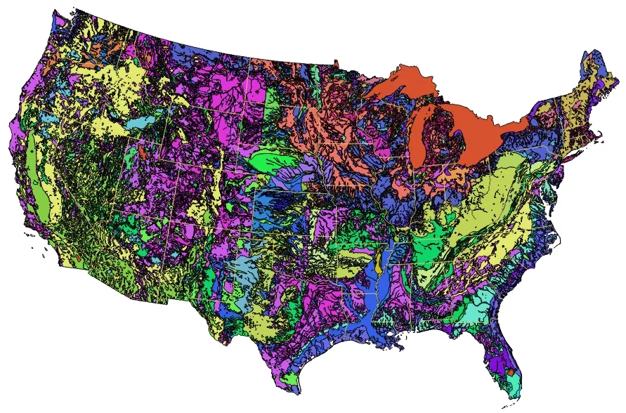

^{1:5,000,000 Surficial Geology Shapefile for the continental US. Features are categorized by Unit Name and are colored randomly.}

You might notice that the colors are a little different than the USGS map, as the styles are not matched. This type of visualization helps with contemplating the complexity of surficial deposit distribution, but the random colors are not very useful for identifying where to look for agates. Before we make those colors more meaningful, there are a couple other useful columns to consider.

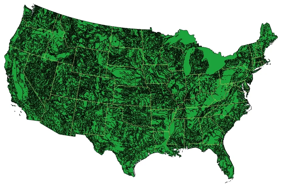
Deposit Thickness

As alluded to earlier, knowing the location of the bedrock geology that Lake Superior Agates are formed in is not entirely helpful in locating the agates. Bedrock is generally obscured by thick deposits of till and glacial outwash in Minnesota, Wisconsin, and Michigan where the Keeweenawan Rift Valley formed. Glacial erosion on this bedrock during the most recent glaciations exposed and transported agates beyond the extent of their source rock. The thickness of surficial deposits can be visualized by styling with the UNIT_THICK column.

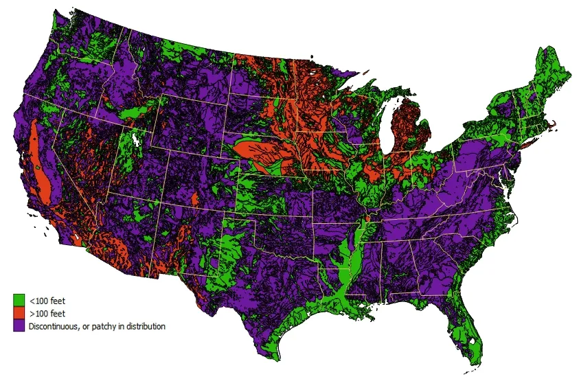
^{Figure 1: 1:5,000,000 Surficial Geology data set showing the thickness of surface material / depth to bedrock with color legend.}

Deposit Age

Another column that might be useful to style the data with is that of UNIT_AGE. Because this data represents a generalized map of the entire country, the time ranges that deposits are lumped into are somewhat broad. Despite this, when the map is styled by 'age' the results are quite interesting:

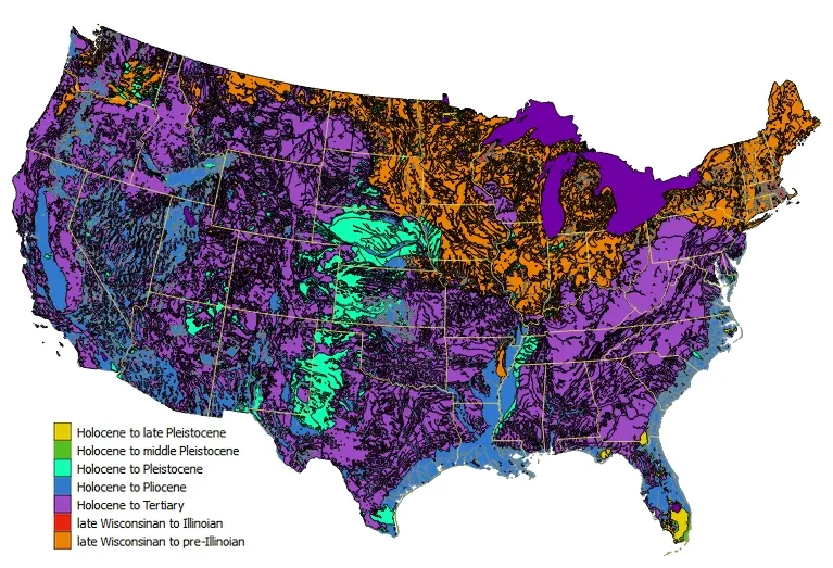
^{1:5,000,000 Surficial geology map styled by 'UNIT_AGE' with legend. All units represent time ranges, and the oldest deposits are cooler colors.}

At first glance, it is clear that the most recent deposits (orange and red) tend to be in the northern part of the country. This corresponds with the Wisconsin and Illinoian stages of glaciation. These are the two most recent glacial events, both occurring within the Holocene. Since we know that the majority of Lake Superior Agates are found in glacial material, we can use the distribution of the orange and red units in the above figure as a rough guide for where to focus our attention.

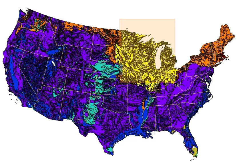
Focusing In

Before proceeding with an analysis of this data in terms of the propensity to possess Lake Superior Agates, it is worthwhile to clip the data set to an area of interest and reduce the overall file size. Though the absolute range of the gemstones is not entirely clear, we can assume that finding the agates is highly unlikely beyond a certain distance from the source rock. As discussed in the previous article, the states of Michigan, Wisconsin, and Minnesota all have the right bedrock to produce agates. If we couple this knowledge with the progression of glaciers during the Holocene, a general search area can be approximated.

Select and Save

The easiest way to filter the data set into an area of interest is to select the desired units with the Select Tool on the Attributes toolbar. This should be turned on by default, but can also be activated through View -> Toolbars -> Attributes. Using this tool we can simply drag a rectangle over Minnesota, Wisconsin, Michigan, and Iowa, as well as parts of Missouri, Illinois, Indiana, and Ohio. The southern limit of Wisconsin and Illinoian deposits serves as a rough southern boundary for the rectangle.

^{Using the Select Tool to create a rough rectangle that highlights the geographic areas most likely to have Lake Superior Agates}

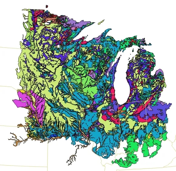
Now that the units of interest are selected, right-click on the 'Surficial_materials' layer and select Save As. In the context menu, select ESRI Shapefile as the file type, give the file a name, and make sure to check Save only selected features. The resultant file, colored randomly by UNIT_NAME, should look something like this:

^{Magnified view showing the units highlighted and exported by our rectangular AOI selection.}

Examining Attributes

Once the data set is whittled down spatially, it becomes much easier to work with. We can begin to consider the individual units and determine how likely each is to contain agates. To see what units remain in our geographic selection, simply expand the layer in the Layers Panel. This acts as a makeshift legend for the map and lists the different classifications of the units being differentiated.

Most units are differentiated in multiple ways - first by deposit type, then by sediment size and deposit thickness. The thickness is not critical in terms of finding agates, but the sediment size is quite useful. In general, silts (Eolian deposits) and the fine sands of proglacial outwash are unlikely to contain gravel-sized agates. Likewise, soil derived from bedrock (residual materials, colluvium) will only contain agates if the local bedrock contains them. Clay-rich deposits like lacustrine, organic muck, and many glacial tills are not the most ideal place to find gravel, but the high energy environment of a glacier can move sediment of all sizes. The best place to look for gravels is in coarse-grained sediment such as alluvial deposits, glaciofluvial outwash, and certain tills that are near the source bedrock. By simply turning off the undesirable units in the Layer Panel, we can start to generate a refined agate map.

Finishing Touches

A final step in optimizing this data is to apply a meaningful color scheme to the polygons. I opted to manually color the remaining units based on the grain size of the deposits and energy of the depositional environments, but a color ramp could also be created or applied as an alternate solution.

Areas with the coarsest sediment and therefore highest probability of finding gravels are highlighted in reds and oranges, while the cooler colors are less ideal. Keep in mind that we have already eliminated the least probable units from the data set, so even cooler colored units have a good chance of containing agates.

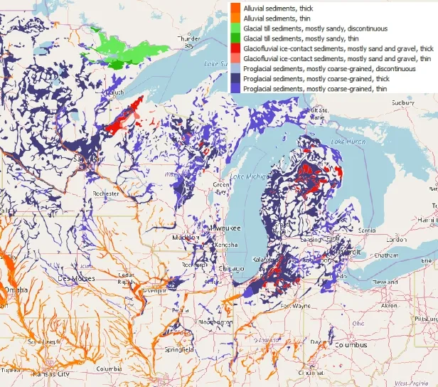
^{Broad overview of color-coded high probability Lake Superior Agate deposits. Basemap by OSM}

The above figure is my best attempt at creating a Lake Superior Agate hunting map using the 1:5,000,000 data. As discussed in the first article in this series, the glacial history that exposed Lake Superior Agates is complex. Unfortunately, this data has no indication of the glacial lobe associated with deposits beyond glacial stages, so we must rely on a spatial estimate. The last article established that the most probable locations to find Lake Superior Agates are in Superior Lobe deposits, which tend to be found in near the Lake Superior basin in Eastern Minnesota, Northern Michigan, and Wisconsin.

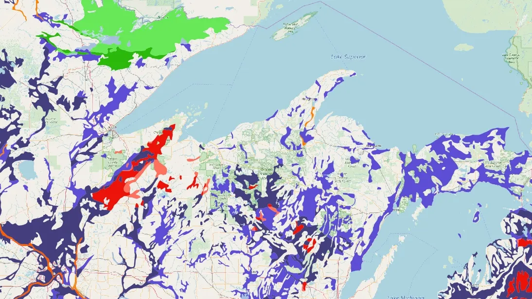^{Magnified color-coded map showing the areas and deposits most likely to contain Lake Superior Agates based on the 1:5,000,000 data. Basemap by OSM}

Improvements

The above graphics provide a first-attempt at locating the most probable locations to look for Lake Superior Agates. There are some obvious setbacks to this data, including the coarse scale and broadly lumped attributes. Nevertheless, I can verify that the map has correctly highlighted some locations in Minnesota that are known to produce agates. While this data can provide some useful insights, these limitations leave some definite room for improvement. The best way to create a better map is to locate better data. Each state has varying degrees of funding and personnel dedicated to mapping surficial deposits, but they all have state-level data available at a better scale than the data set utilized in this article.

Minnesota even has detailed aggregate maps at the county level up to a scale of 1:24,000! Once this data is massaged and processed in the right way, it has the capacity to precisely identify where to find agates - down to the scale of individual gravel pits and creeks. Truth be told, this detailed analysis on high-resolution data has already been performed and distilled into a powerful map-based tool that can be accessed from any device. If you are interested in rockhounding and want to use the best information available to gain an edge on the competition, contact me on discord! Happy hounding!

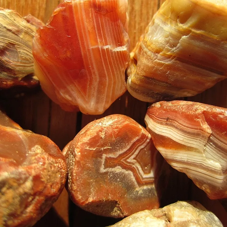
^{A small sampling of agates discovered through GIS.}

External References

[a] - Soller, D.R., Reheis, M.C., Garrity, C.P., and Van Sistine, D.R., 2009, Map database for surficial materials in the conterminous United States: U.S. Geological Survey Data Series 425, scale 1:5,000,000 [https://pubs.usgs.gov/ds/425/].
Huber, N K. The Keweenawan geology of Isle Royale, Michigan. US Geological Survey, 1971. [https://pubs.er.usgs.gov/publication/ofr71154]
Huber, N K. The Geologic Story of Isle Royale National Park. US Geological Survey, 1975. [https://pubs.er.usgs.gov/publication/b1309]
QGIS Development Team (2018). QGIS Geographic Information System. Open Source Geospatial Foundation Project. http://qgis.osgeo.org".

Thank you for reading my article! All photos are by the author unless otherwise noted. See additional reading and references as hyperlinks within the text. If you enjoy reading and writing original, high-quality science, technology, engineering, and math posts on the Steemit blockchain, you should really check out @steemstem! For more information on what a steemSTEM post should contain, see HERE and check out pinned messages in the official Discord Server! Here they even have a great team of honor members who can answer your questions and offer mentoring!

Making Spatial Data Yield Agates