In this blog post I want to do two things that I haven't done for a long time. I am going to blog about nutrition, and I'm going to write this blog using Jupyter Notebook an Python.
This blog is both menat to be informational regarding macros from a nutritional perspective, and I'm going to walk you through the process of looking at the theory with Python and Jupyter notebook in a way that makes this a little bit of a tutorial.
In order to use Jupyter for the things we wnt to do today, the first thing we need to do is import a few python libraries.
import matplotlib
import numpy as np
import pandas as pd
import math
%matplotlib inline
The numpy library is an amazing Python library for working with arrays.
Pandas extends on numpy by providing what basically results in an in-code spreadsheet.
Think of pandas, especialy when running inside of Jupyter, as excel on steroids.
The matplotlib is a library that is used to plot the data and visualize our findings.
Now that we have our base requirements, it is time to look at some nutrition equations and put them into Python functions.
We are going to start odd looking at a few well known formulas from nutrition. The first one is the Katch-McArdle equation for daily energy expendature.
It takes two variables. the lean body mass of the person. This is the total body mass minus the weight of the adipose tissue, and a so called activity factor that is an indication of how active a person is.
| how active | activity factor |
|---|---|
| sedentary | 1.2 |
| light activity | 1.375 |
| moderate activity | 1.55 |
| high activity | 1.725 |
| extreme activity | 1.9 |
The second equation uses a timplified version of one of two often used rule ot thumb.
- 1 gram of protein per lbs of lean body mass
- 2.5 grams of protein per kg of lean body mass
There are other equations sometimes being used using total body mass with a lower number for protein intake per kg ranging from as low as 0.8 gram per kg (though that number usually comes from people with an animal right of vegan background) up to 2 gram per kg.
For this blog, knowing that the energy content of 1 gram of protein equates 4 kcal, we are going with the second statement for out second equation.

The ideal total protein-sourced energy intake is 10 kcal per kg of lean body mass.
Now we need to pick sides. Do we want to go low fat, low carb, or somewhere in between. Looking at development in nutrition in recent decades, and ignoring the animal rights tainted vegans for a bit, we are going for low carb for this blog. There are different definitions of what would constitute low carb, and we both want to take the concept serious and steer away from the absolute zero idea that might be a bit extreme. We pick the often cited number of 50 grams, or 200 kcal from carbohydrates.
Then finaly, fat. If we wanted to be complete we would add alcohol to the list because its another source of energy for many of us, but to keep this blog simple, we assume that all calories not from either protein nor carbohydrates come from fat.
So lets express this in Python
def katch_mcardle(lbm, activity):
    return (370 + 23.6 * lbm) * activity

def protein_kcal(lbm, activity):
    return 10*lbm

def carb_kcal(lbm, activity):
    return 200

def fat_kcal(lbm, activity):
    return (katch_mcardle(lbm, activity) -
            protein_kcal(lbm, activity) -
            carb_kcal(lbm, activity))
Now lets look a little bit into numpy, pandas and the posibilities to plot data.
We start off with a simple function calculating the ideal percentage of calories that should come from protein.
def protein_pct_kcal(lbm, activity):
    return 100 * protein_kcal(lbm, activity) / katch_mcardle(lbm, activity)
Let's demonstrate. We take a lean body mass of 70 kg for a sedentary person (activity 1.2) and look what we get.
protein_pct_kcal(70,1.2)
28.84932410154962
The protein_pct_kcal function takes two arguments, the lean body mass and the activity factor.
Let's say we need a function that takes just the lean body mass as argument. We can make such a function using Python't lambda expressions.
sedentary_pct_kcal = lambda x : protein_pct_kcal(x, 1.2)
sedentary_pct_kcal(70)
28.84932410154962
It is good to be able to get the result of this function for just one value of lbm. But when we want to plot a graph, we want to do so for a collection of values.
For this the numpy offers two things: The linspace with what we can define a range of equally spaced input values, and the vectorize feature that allows us to turn a function that takes a scalar as argument into a function that takes an array as input instead and calculated all the results at once.
We start off defining a linspace ranging from 20 kg till 90 kg for our lean body mass.
lbm = np.linspace(20,90,71)
lbm
array([20., 21., 22., 23., 24., 25., 26., 27., 28., 29., 30., 31., 32.,
       33., 34., 35., 36., 37., 38., 39., 40., 41., 42., 43., 44., 45.,
       46., 47., 48., 49., 50., 51., 52., 53., 54., 55., 56., 57., 58.,
       59., 60., 61., 62., 63., 64., 65., 66., 67., 68., 69., 70., 71.,
       72., 73., 74., 75., 76., 77., 78., 79., 80., 81., 82., 83., 84.,
       85., 86., 87., 88., 89., 90.])
Finaly we vectorize the function and invoke it with our linspace lbm array
vectorized_sedentary_pct_kcal = np.vectorize(lambda x : protein_pct_kcal(x, 1.2))
vectorized_sedentary_pct_kcal(lbm)
array([19.79414093, 20.21719039, 20.61778378, 20.99766287, 21.35839385,
       21.70138889, 22.02792463, 22.33915806, 22.63614021, 22.91982802,
       23.19109462, 23.45073832, 23.69949046, 23.93802228, 24.16695098,
       24.38684504, 24.59822893, 24.8015873 , 24.9973687 , 25.18598884,
       25.36783359, 25.54326156, 25.71260652, 25.87617947, 26.03427057,
       26.18715084, 26.33507374, 26.47827655, 26.61698163, 26.75139762,
       26.88172043, 27.00813421, 27.13081225, 27.24991774, 27.36560448,
       27.47801759, 27.58729408, 27.69356343, 27.79694809, 27.89756393,
       27.99552072, 28.09092249, 28.18386792, 28.27445067, 28.3627597 ,
       28.44887955, 28.53289064, 28.61486948, 28.69488893, 28.77301841,
       28.8493241 , 28.92386912, 28.99671371, 29.06791539, 29.13752914,
       29.20560748, 29.27220065, 29.33735674, 29.40112177, 29.4635398 ,
       29.52465309, 29.5845021 , 29.64312569, 29.70056109, 29.75684407,
       29.81200898, 29.86608879, 29.91911522, 29.97111874, 30.02212867,
       30.07217322])
So far we have been using raw numpy arrays. Fr our purpose though it is usefull to switch to using pandas dataframes.
Think of a dataframe like a spreadsheet. Let's put our lbm linespace into one column of this spreadsheet and then put the result of our vectorized version of our function into a second column.
df1 = pd.DataFrame()
df1["lbm"] = np.linspace(20,90,71)
df1["sedentary"] = np.vectorize(lambda x : protein_pct_kcal(x, 1.2))(df1["lbm"])
df1.head(10)
| lbm | sedentary | |
|---|---|---|
| 0 | 20.0 | 19.794141 |
| 1 | 21.0 | 20.217190 |
| 2 | 22.0 | 20.617784 |
| 3 | 23.0 | 20.997663 |
| 4 | 24.0 | 21.358394 |
| 5 | 25.0 | 21.701389 |
| 6 | 26.0 | 22.027925 |
| 7 | 27.0 | 22.339158 |
| 8 | 28.0 | 22.636140 |
| 9 | 29.0 | 22.919828 |
df1["light"] = np.vectorize(lambda x : protein_pct_kcal(x, 1.375))(df1["lbm"])
df1["moderate"] = np.vectorize(lambda x : protein_pct_kcal(x, 1.55))(df1["lbm"])
df1["very"] = np.vectorize(lambda x : protein_pct_kcal(x, 1.725))(df1["lbm"])
df1["extremely"] = np.vectorize(lambda x : protein_pct_kcal(x, 1.9))(df1["lbm"])
df1.head(10)
| lbm | sedentary | light | moderate | very | extremely | |
|---|---|---|---|---|---|---|
| 0 | 20.0 | 19.794141 | 17.274887 | 15.324496 | 13.769837 | 12.501563 |
| 1 | 21.0 | 20.217190 | 17.644093 | 15.652018 | 14.064132 | 12.768752 |
| 2 | 22.0 | 20.617784 | 17.993702 | 15.962155 | 14.342806 | 13.021758 |
| 3 | 23.0 | 20.997663 | 18.325233 | 16.256255 | 14.607070 | 13.261682 |
| 4 | 24.0 | 21.358394 | 18.640053 | 16.535531 | 14.858013 | 13.489512 |
| 5 | 25.0 | 21.701389 | 18.939394 | 16.801075 | 15.096618 | 13.706140 |
| 6 | 26.0 | 22.027925 | 19.224371 | 17.053877 | 15.323774 | 13.912373 |
| 7 | 27.0 | 22.339158 | 19.495992 | 17.294832 | 15.540284 | 14.108942 |
| 8 | 28.0 | 22.636140 | 19.755177 | 17.524754 | 15.746880 | 14.296510 |
| 9 | 29.0 | 22.919828 | 20.002759 | 17.744383 | 15.944228 | 14.475681 |
Looks pretty good already, but let's make lbm our row index.
df1.set_index("lbm", inplace=True)
df1.head(10)
| sedentary | light | moderate | very | extremely | |
|---|---|---|---|---|---|
| lbm | |||||
| 20.0 | 19.794141 | 17.274887 | 15.324496 | 13.769837 | 12.501563 |
| 21.0 | 20.217190 | 17.644093 | 15.652018 | 14.064132 | 12.768752 |
| 22.0 | 20.617784 | 17.993702 | 15.962155 | 14.342806 | 13.021758 |
| 23.0 | 20.997663 | 18.325233 | 16.256255 | 14.607070 | 13.261682 |
| 24.0 | 21.358394 | 18.640053 | 16.535531 | 14.858013 | 13.489512 |
| 25.0 | 21.701389 | 18.939394 | 16.801075 | 15.096618 | 13.706140 |
| 26.0 | 22.027925 | 19.224371 | 17.053877 | 15.323774 | 13.912373 |
| 27.0 | 22.339158 | 19.495992 | 17.294832 | 15.540284 | 14.108942 |
| 28.0 | 22.636140 | 19.755177 | 17.524754 | 15.746880 | 14.296510 |
| 29.0 | 22.919828 | 20.002759 | 17.744383 | 15.944228 | 14.475681 |
Now it's time to call in matplotlib
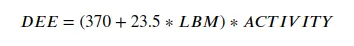
df1.plot(grid=True)
<AxesSubplot:xlabel='lbm'>
We see that extremely active people with a really low lean body massshould have enugh consuming less than 15% of calories from protein, while sedentary people with extemely high lean body mass should consume double taht percentage. It is clear to see that there is no one size fits all here.
We all know counting calories is a drag, and many claim its a bad idea, and its hard not to agree. Lets take one step towards not counting calories by for now just counting grams instead.
Both protein anf carbohydrated have roughtly 4 kcal per gram and fat about 9 kcal.
def protein_grams(lbm, activity):
    return protein_kcal(lbm, activity) / 4.0

def carb_grams(lbm, activity):
    return carb_kcal(lbm, activity) / 4.0

def fat_grams(lbm, activity):
    return fat_kcal(lbm, activity) / 9.0
We do the same as we did before, but now with grams instead of kcal. Lets start off with our function.
def protein_pct_gram(lbm, activity):
    return (100 * protein_grams(lbm, activity) /
            (protein_grams(lbm, activity) +
             carb_grams(lbm, activity) +
             fat_grams(lbm, activity)))
The rest is pretty much the same as before
df2 = pd.DataFrame()
df2["lbm"] = np.linspace(20,90,71)
df2["sedentary"] = np.vectorize(lambda x : protein_pct_gram(x, 1.2))(df2["lbm"])
df2["light"] = np.vectorize(lambda x : protein_pct_gram(x, 1.375))(df2["lbm"])
df2["moderate"] = np.vectorize(lambda x : protein_pct_gram(x, 1.55))(df2["lbm"])
df2["very"] = np.vectorize(lambda x : protein_pct_gram(x, 1.725))(df2["lbm"])
df2["extremely"] = np.vectorize(lambda x : protein_pct_gram(x, 1.9))(df2["lbm"])
df2.set_index("lbm", inplace=True)
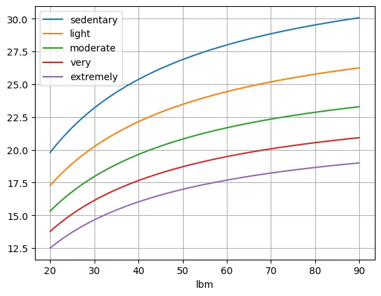
df2.plot(grid=True)
<AxesSubplot:xlabel='lbm'>
Notice that all the numbers are a little bit higher. This stems from the higher energy density of fat.
Now let's take our road away from counting calories one step further. Let's look at out fat to protein ratio and see how that comes out.
def fat_to_protein_ratio(lbm, activity):
return fat_grams(lbm, activity) / protein_grams(lbm, activity)
df3 = pd.DataFrame()
df3["lbm"] = np.linspace(20,90,71)
df3["sedentary"] = np.vectorize(lambda x : fat_to_protein_ratio(x, 1.2))(df3["lbm"])
df3["light"] = np.vectorize(lambda x : fat_to_protein_ratio(x, 1.375))(df3["lbm"])
df3["moderate"] = np.vectorize(lambda x : fat_to_protein_ratio(x, 1.55))(df3["lbm"])
df3["very"] = np.vectorize(lambda x : fat_to_protein_ratio(x, 1.725))(df3["lbm"])
df3["extremely"] = np.vectorize(lambda x : fat_to_protein_ratio(x, 1.9))(df3["lbm"])
df3.set_index("lbm", inplace=True)
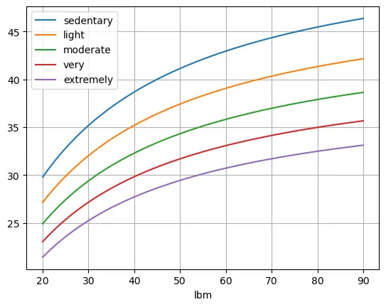
df3.plot(grid=True)
<AxesSubplot:xlabel='lbm'>
Things get a little interesting now.We are seeing while lean body mass definetely has an impact on the ideal ratio, the activity factor is most leading. For sedentary people, a fat to protein ratio of roughly one seems to be OK, adding in some extra fat for people with really low body fat.
For extremely active individuals though, something closer to a ratio of two grams of fat for every fram of protein makes a lot of sense.
I hope this little walktrhough on using numpy, pandas and matplotlib in Jupyter notebook to visualize some basic theory and assumptions has been usefull for you as a reader, and for those of you less interested in that part of the subject, I hope the resulting graphs have given you some insights in this aspect of nutrition.