
Source: Pixabay, CCO licensed
Disclaimer: The reason I wrote this post is that I enjoyed doing so, the challenge to create a good post about one subject I like is enough fuel for me to try... I'm far from being an expert in this field but I enjoyed the research I needed to conduct in order to grasp the basics of the subject. The key concepts and the workflow of the following ideas are based on the first chapter of the book: "Fundamentals of Quantum Chemistry", Molecular Spectroscopy and Modern Electronic Structure Computations, M. Mueller, Kluwer Academic Publishers, 2001.
The foundations of Classical Mechanics are what we could label as everyday experiences, through careful observations scientists made a theoretical model capable of explaining macroscopic phenomena and quantitatively describing it's properties. One key concept needed to be understood is that of a "particle", a particle is a small object which position and speed can be determined with the only limitations of those arising from the uncertainty of the instruments used to measure the particle's properties. The key idea here is that in Classical Mechanics if we can know all the forces acting on the particle, then we can determine precisely where a particle is as well as determine it's motion trajectory.
Now we know this is not true on a microscopic scale, but the results yielded by Classical Mechanics apply so successfully to the bulk scale that the quantum theory has to converge with Classical Mechanics results when we treat macroscopic phenomena. From the Newtonian law of motion, we have that for any inertial reference frame the second derivative of the position times the mass of the particle equals the resultant force acting on the particle:
Here, F = resultant force, m = mass of the particle, the q with two dots stands for the second derivative of the position in a cartesian, polar or spherical inertial coordinate frame. Most of us are very familiar with the standard approach to solving Classical Mechanics problems. We break the Resultant Force vector into its components in our reference frame, then we solve each component individually and finally add them up using the additive properties of vectors. These types of problems often yield differential equations system which in some cases can be readily integrated.
Hamiltonian Mechanics
In 1834, the Scottish mathematician William R. Hamilton developed a method under which some complex problems could be solved. In order to grasp the Hamiltonian approach, we have to recall that a conservative system is one in which the forces acting over an object don't vary as time passes, i.e. those forces are just functions of the position of the aftermentioned object. Examples of such conservative forces are the gravity force and the electric force. Since they are functions of a characteristic magnitude of the interacting objects (i.e. mass and electric charge) and the distance between them. A non-conservative force usually is a dissipative one (i.e. they dissipate energy) such as frictional forces.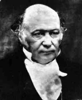
m=mass, r=distance between masses
G=Foundamental gracity constant
q=charge, r=distance between charges
k=Foundamental electric constant
Another important concept is that of generalized coordinates, a regular coordinate system describes the position of a point in the space by stating the distance to this object from an arbitrary point called the origin. Thus, if we have a particle in a plane, we can describe its position as "x" horizontal units away from the origin and "y" vertical units away from the said origin. The utility of generalized systems is that there are times when the position of an object requires fewer points from what this regular coordinates offer, thus we can describe that object's position in a more simpler and compact set of coordinates called "generalized coordinates".
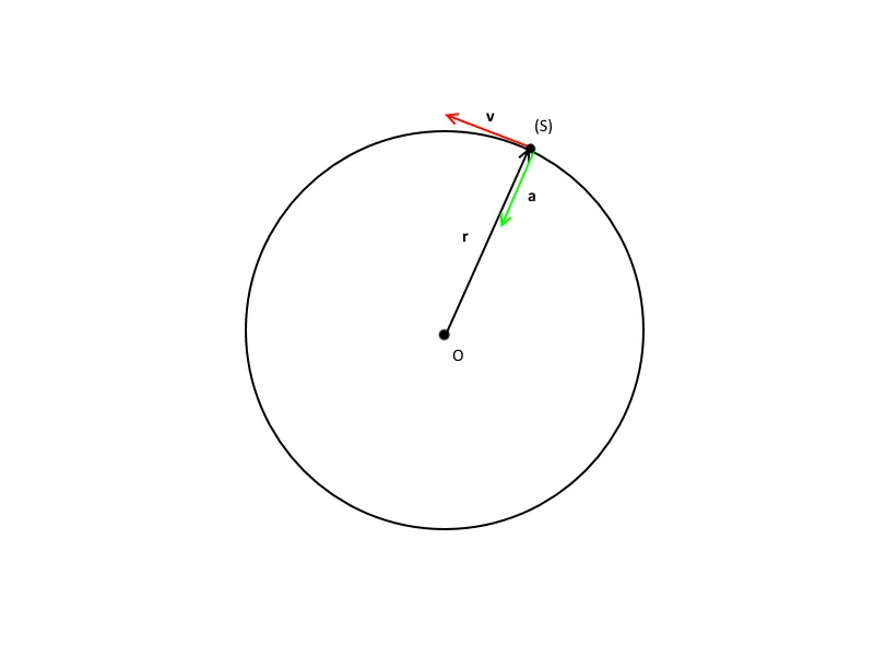
For instance, let's think about a particle moving on a circle in a 2D plane, we could use x and y coordinates to describe its motion, but we don't need to. The particle is constrained to move on the circular trajectory, hence we can just state the radius from the center of the circle and formulate the angle it covers as a function of time. Thereafter, the particle's movement will be perfectly described using a constant (the radius) and a single variable (the angle) instead of two cartesian variables.
In general, an ordinary n-dimensional coordinate system would require "n" individual variables to describe the position of each particle within it, while the generalized coordinates system would require that for "n" dimensions, "m" particles moving under "k" constraints a total of mb-k generalized coordinates.
With these concepts clearly understood, we can inspect next the definition of the Hamiltonian for a particle (or a lot of particles) under the effects of conservative forces:

Equation 1
Here H is the Hamiltonian, T is obtained from the kinetic energy of the system and V from the potential energy.
The Kinetic Energy of a particle is usually defined as the product of the mass times the half of the square of the velocity, but we shall define it as the dot product of the momentum vector divided by two times the mass of each particle. The potential energy only depends on the positions of each particle and it's usually the trickiest part of writing the Hamiltonian.
Equation 2
For these types of systems, Hamilton proposed that for a generalized coordinate frame, the motion equations can be obtained from the Hamiltonian and the following identities:
The Hamiltonian in action
Let's consider a vertical thrown particle of mass m:

Gif made by the author using picasion.com and Microsoft PowerPoint
Also, let's first solve the problem using the Newtonian mechanics:
Since the motion takes place alongside a line, we can consider it unidimensional, thus we can take vectorial magnitudes as scalar ones.
After integrating two times with respect to the variable "t" (the time) we get the familiar result:
Let's see how we can handle this using the Hamiltonian, we have to make an expression for the kinetic energy of the particle in terms of its momentum plus its potential energy.
Afterwards, we take the partial derivative of the Hamiltonian with respect to the particle's coordinates and consider it's momentum constant, we get:
Then we pay attention to the partial derivate of the Hamiltonian with respect to the particle's momentum and considered its coordinate variables constant.
Since this example is extremely simple, here we get a trivial relationship because the momentum is just the product of the velocity times the mass of the particle, but it is this capability to consider the momentum of the particle independent of its coordinates the feature which makes the Hamiltonian so useful in quantum mechanics (later we'll handle fairly complex examples where the usefulness of the Hamiltonian will be clearly appreciated).
Ok, but this seems like a Physics class, what's the relationship with Chemistry?
Well, it turns out that variables governing the Harmonic oscillator can be readily described using the Hamiltonian, this Harmonic Oscillator model is a fundamental tool to describe the vibrational energy alongside the chemical bond between the atoms in a molecule.
Let's consider first the simple model where one of the ends of the spring is attached to a fixed location and the other end is attached to a particle of mass m (This model yields good results when the mass of one atom in a diatomic molecule which greatly exceeds the mass of the other, such as Hydrogen Bromide). The mass is bound to move only on the x axis and it will have potential energy according to Hook's law.
Gif made by the author using gifmaker.me and Microsoft PowerPoint
The Hamiltonian for such system is of the form:
When we take the partial derivative of the Hamiltonian on equation 4 we get:
Then we can notice that the derivative on equation 5 produces a trivial result since the momentum is just the velocity times the mass:
The first derivative allows us to find the trajectory of the particle since the first derivative of the momentum is just the resultant force, or the mass times the acceleration, thus we have:
Equation 5
The solution to this differential equation is well known

Equation 6
It also can be written using imaginary numbers as
Equation 7
Taking a closer look to the above equations, we can know that xo is the equilibrium point of the spring (the initial position), also we notice that omega must have units of the inverse of time since the exponential, sine, and cosine functions should have dimensionless arguments. Furthermore, we can state that this omega is related to the oscillation frequency of the spring. To have an explicit expression for omega we can take the second derivative of both the equation 6 or equation 7 to get:
Equation 8
From equation 5 and equation 8 we get an expression for omega (the oscillation frequency) in terms of the variables of our model:
 From the fact that the cosine and sine functions oscillate from -1 to 1, the constants (a, b, A, B) on equation 6 and equation 7 are related to the amplitude and the phase of the oscillation. Since we haven't quantized this model yet, there are no constraints for the values of these constants... but the fact that in molecular bonds these constants have a limited set of allowed values, because of the spacial constraints caused by the other bonds and atoms in the surroundings, and because of the nature of the bond itself (for instance simple bonds and double bonds vibration is not the same alongside two carbon atoms), we can identify the identity of the bonds present in a sample via infrared spectroscopy (On this technique, a device called infrared spectrometer is used to apply infrared radiation -the radiation between 0.7-1000 μm, the resulting spectra allow us to identify which bonds are present in the sample since the wavelength absorption range is a unique characteristic of each bond).
Let's see how the scope of the Harmonic Oscillator model can be broadened
Let's remove the limitation of one mas being greater than the other to describe better diatomic molecules.
Gif made by the author using gifmaker.me and Microsoft PowerPoint
Now, we will consider two masses m1 and m2 separated by a string with a force constant k and equilibrium length xo. We shall see here how taking generalized coordinates instead of ordinary coordinates allows us to simplify the equations.
Gif made by the author using gifmaker.me and Microsoft PowerPoint
The Hamiltonian for such configuration of masses is as follows:
Equation 9
This Hamiltonian is not as easy to solve as the previous ones, but if we can introduce some convenient generalized coordinates we can simplify it. Let's define r as the length of the spring outside from its equilibrium length and let s be the position of the mass center of the system.

After introducing these simplifications, the potential energy of the system becomes into the product of half the elastic constant times r square (the new coordinate for the displacement of the string from its equilibrium point). After this, we have to transform the momentum using the new coordinates taking the derivative of r and s with respect to the time:
Equation 10
Equation 11
From equation 10 and equation 11 we can find expressions for the time derivative of X1 and X2 with respect to the time (the velocities).
Equation 12
Equation 13
From the last two equations, we can create expressions for the momentum of the system in terms of the generalized coordinates:
Further simplification can be made if we define the reduced mass "μ" of this system as the term in parenthesis in the above couple of equations.
Equation 12
Equation 13
Now we can merge all these expressions into our Hamiltonian to get:

Since "s" is the generalized coordinate for the center of mass, we can assume that the momentum of this coordinate corresponds to the translational kinetic energy. Because we are only interested in the vibrational energy, our final Hamiltonian has the form:
Our generalized coordinates have proven useful, now we can recognize the shape of this last Hamiltonian as the one we solved previously for the Harmonic Oscillator, thus the solution for this one is also of the form:

This solution grants us a glimpse of how Classical Mechanics concepts lead us to the doorstep of solving atomic problems, the main goal of this article was to emphasize the usefulness of the Hamiltonian and the generalized coordinates to solve otherwise complicate equations and to lay the foundations to comprehend quantum phenomena. In the next part, we shall discuss a little bit of the fundamental ideas of Quantum Mechanics and how these concepts are applied to describe better properties of atoms and molecules from a chemist's perspective.
我好朋友 @davidke20让我知道我是否解释好了这篇文章。
All equations were made on codecogs.com latex online editor.