Most discussions about human carbon emissions are centered around the idea of the greenhouse effect and climate change, whether you agree with it or not. But did you now that our addiction to fuel combustion has even more implications? Some might even be familiar with ocean acidification for example, where increased CO2 concentrations allow more gas to be dissolved and increase the acidity of the oceans. But also the way archaeologist perform research can be thrown upside down because of this.
A commonly used way to date organic material is based on the different types (isotopes) of carbon in the environment. It allows to date once-living materials of at least 100 years, up to 50.000 years old. You might also know it as carbon dating or c-14 dating. Because we emit 9.000.000.000 tons of carbon in the atmosphere each year, the natural balance of different carbon isotopes is distorted which impacts the accuracy of this carbon dating method.
I will give an overview of how carbon dating works followed by the way in which our emissions have an effect on archeology. It is not my attempt to give you a degree in atomic sciences or make you an archaeologist so I might simplify for the sake of a clear explanation. I will provide links throughout the text to more in depth explanations of the concepts addressed here.
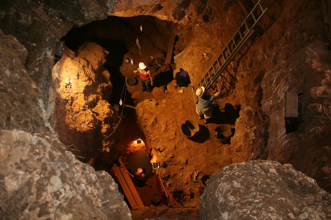
Archeological excavation in Santa Ana Cave, Spain. Image by Mario Modesto Mata, shared under Creative Commons Attribution-Share Alike 3.0
Introduction to carbon dating
Natural balance of carbon isotopes
Atoms exist of protons, neutrons and electrons. And since the type of element is determined by the amount of protons, varieties can exist between different atoms of a same element, these varieties are called isotopes. Carbon for example has 6 protons and the average weight of the atom is 12.0107. Meaning that on average there are 6 more neutrons in the core. It is possible for carbon to contain more neutrons, for example 7 or 8. An isotope having 7 neutrons in the core is still stable but a carbon atom with 8 neutrons is radioactive and will decay. This atom has a weight of 14 (8 neutrons + 6 protons) and is therefor called 14C (C-14). This 14C has a half-life of 5.700 (+- 30) years, meaning 50% will decay into Nitrogen (14N ) in about 5.700 years.
Because this is an unstable isotope, you wouldn't expect much of it to be around. In the atmosphere however, at an altitude of 9 to 15 kilometers, cosmic radiation interacts with existing nitrogen atoms, transforming 14N into 14C . This constant production of 14C from 14N, combined with a constant decay of 14C back into 14N leads to a natural balance between the 14C concentration and the stable12C concentration. Approximately one 14C atom exists for every trillion 12C atoms.
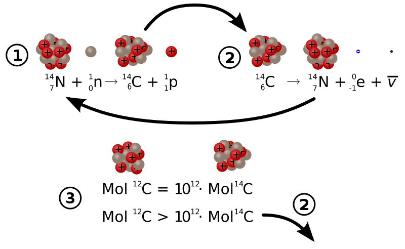
The physics of carbon 14 decay and creation. 1) indicates 14C creation from 14N and cosmic radiation, 2) indicates the radioactive decay of 14C and 3) shows the approximate concentrations of the different isotopes. Illustration by Sgbeer, shared under attribution-share alike 3.0 licence.
Deriving age from this balance
Gas particles in the atmosphere are assumed to mix relatively fast compared to the decay rate of carbon 14. So if the carbon atom with a weight of 14 reacts with an oxygen atom to form CO2, after which it is absorbed by an organism at the surface, it is a decent assumption to assume that this organism also has the same balance of 14C and 12C in its body as present in the atmosphere. Throughout its entire lifetime organisms exchange carbon with the environment so as long as it is alive, the balance is almost identical to the balance of the atmosphere.
When the organism dies however, it stops exchanging carbon atoms with the environment. Only decay of 14C can continue to take place. Lets say you find a piece of wood of an unknown age deep under the ground. You could measure the radioactive emission coming from carbon 14 atoms. If you find that the activity is half of what you would expect from atmospheric 14C concentrations, you can conclude that your piece of wood is about 5.700 years old. Notice that the age you measure is the age when the organism stopped exchanging carbon with its environment! So you measure the time of death. This is often important in making conclusions about your data.
Natural fluctuations in the 14C concentrations
Throughout history many effects have influenced the balance of 14C creation. For example in periods of a weaker magnetic field or increased solar activity, more cosmic radiation could reach the atmosphere and more N14 could be converted to 14C . This can cause in an over- or under estimation of carbon age. Let me make it clear with an example. Imagine that cosmic activity is twice as high, and the 14C concentrations are twice as high as well. A tree that died in that period, would have the same radio active activity as a tree that died 5.700 years later in normal conditions. Because of this the old tree would have been measured 5.700 years younger than it actually was because of fluctuations in cosmic activity. It also works the other way around in time periods with lower 14C concentrations. A carbon sample can look like it has already decayed a long time, while the atmospheric concentrations were just low to begin with.
To resolve this problem, people created curves to correct for these fluctuations. They managed to derive precise 14C concentrations of things with known age (such as tree rings) and construct a graph for calibration.
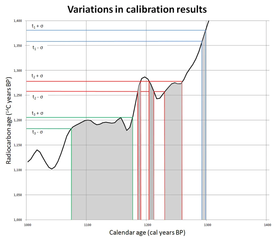
variations in calibration results. On the Y axis you have the measured age according to the current 14C activity and the constant half-life of 5700 years. The colored lines indicate the probability of a certain age, they are equal for all three examples. By projecting the measured ages on the curve, you can read the calibrated calendar ages of your measurements on the X-axis. It is immediately clear that depending on the atmospheric conditions at the time of your sample, your calibrated age can change significantly. Graph from Mike Christie shared under attribution-share alike 3.0.
If a constant concentration of 14C was present in the atmosphere we would expect a straight line of 45 degrees and projected carbon ages are the same as the measured carbon ages. a sudden decrease of 14C concentration would lead to a flattening of the curve. If we follow the example of the tree from earlier, a piece of organic material measured to be 10.000 years old could be from the youngest tree, or from the tree that was 5.700 years older. The older tree had twice the 14C amount when it died, but the 14C had already 5.700 years to decay. A sudden increase in 14C concentration improves the accuracy.
How humans influence carbon dating
The fossil fuels we commonly burn, and are a major part of antropogene carbon emissions, are actually organic compounds as well. Only these are far older than 50.000 years and carbon 14 is as good as absent. When we release these carbon atoms in the form of CO2, we strongly dilute the concentration of14C . In the past 50 years we have increased the amount of carbon dioxide by almost 30% (from 320 ppm in 1960 to 410 ppm in 2018). When you read the last paragraph of the previous section again, you can conclude that this would result in a flattening of the calibration curve and an increase of uncertainty in radio carbon dates.
Another way to understand this goes as follows. When an organism dies, 14C concentrations drop because of decay. But when 14C concentrations in the atmosphere drop as well, it will become difficult to distinguish when the organism stopped exchanging 14C with its environment. If the 14C decrease is equally fast as the decay rate it would even become impossible to determine when it stopped exchanging carbon with the environment.
A dedicated study on the subject by Heather D. Graven determined that at this rate, in 2050 organic material will appear 1.000 years old, corresponding to an aging rate of 30 years per year. 14C concentrations are thus declining faster in the atmosphere than they would when only decay plays a role.
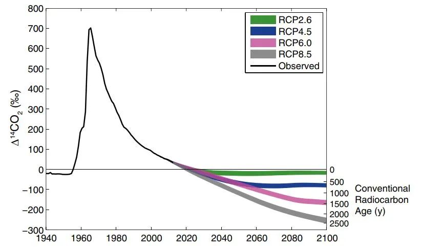
Observed and modeled measured radio carbon ages for atmospheric 14C concentrations. Notice the peak after 1960 because of nuclear testing (more in discussion). Graph from Graven (2015).
Conclusion
It is also interesting to note that human activities also influenced this phenomenon in the other direction. Due to nuclear bombs and testing, cosmic radiation is imitated. According to literature, atmospheric 14C concentrations would have almost doubled between 1950 and 1960. But because the carbon cycle has large sinks, this peak declined after a few decades as you can see on the previous figure.
Although very popular, carbon dating is not the only method to date stuff. There exist many other isotopes that can be used for the purpose and not all dating techniques require isotopes. But at current trends carbon dating seems to be inaccurate when objects from this era are measured. Luckily we live in a society filled to the brim with information and at least for the archaeologist of the future there will be other ways to determine the age of something. Perhaps when an object is made from plastic or cannot connect to WiFi yet, future researchers can identify it to this time period.
I hope I could show you something new to day! Feel free to make any comments on my writing or leave your opinion. I would love to hear from you!
Sources
Graven, H. D. (2015). Impact of fossil fuel emissions on atmospheric radiocarbon and various applications of radiocarbon over this century. Proceedings of the National Academy of Sciences, 112(31), 9542–9545. https://doi.org/10.1073/pnas.1504467112
https://theconversation.com/explainer-what-is-radiocarbon-dating-and-how-does-it-work-9690
https://www.radiocarbon.com/tree-ring-calibration.htm
https://www.radiocarbon.com/carbon-dating-bomb-carbon.htm
https://en.wikipedia.org/wiki/Carbon-14
https://en.wikipedia.org/wiki/Radioactive_decay
https://en.wikipedia.org/wiki/Radiocarbon_dating_considerations