This is an addendum to my previous post which you can see here: https://steemit.com/steemstem/@dexterdev/studying-global-motions-of-proteins-from-molecular-dynamics-trajectories
Repository
https://github.com/dexterdev/STEEMIT/blob/master/FLUCTUATIONS
PCA caveat
From PCA plots it is possible to create normalized histograms or distribution plots based on the density of scatter plot dots. Also, people sometimes convert those distributions to "free-energy "calculations. Of course, they are not the real free-energy measures, but a dimensionally reduced and okay-to-use practical measure. More about those caveats later.
Another point which deserves noticing is about the usage of PCA itself as a dimensionality reduction technique. As @alexs1320 mentioned in my last post here:
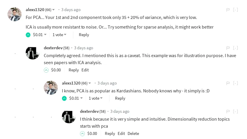
Yes PCA is as popular as Kardashians! :P
There are improved alternative techniques like:
- dPCA (dihedral PCA)
- ICA (Independent component analysis)
- tSNE and others
More about those techniques in the future.
Tracking the molecule in time through the PC space
I just wrote a code in MATLAB to temporally and spatially track the simulation structures in the principal component space.
CODE: https://github.com/dexterdev/STEEMIT/blob/master/FLUCTUATIONS/video_PC_tracker.m
This code uses mtit.m file from here.
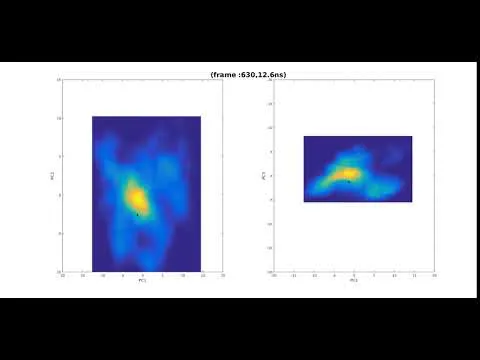
The black dot in the youtube video represents the protein structure(CA atoms). As it changes the structure it moves through the PC space. The yellowish regions are the regions where protein like to visit more often. It can be thought of a local minima in free energy space.
CODE:
close, clear,clc

PC=load('./PC_all_combined_ubq-fitted.dat') ;


t=0;

targetframerate = 24;
frametime = 1/(24*60*60*targetframerate);
nextframe = now + frametime;
tic
nframes = 1;


hFig = figure('Visible','off','Position', [100, 100, 1920,1080]);
set(hFig, 'PaperPositionMode','auto')

%str=strcat(datestr(clock,'dd-mmm-yyyy HH:MM:SS'),'_nbpm_3_4','_T_',num2str(T/60));
str = 'PC1_PC2_PC3_tracker';

writerObj = VideoWriter(str);
open(writerObj);
for frame = 1:10:1250
    ht.String = ['Time = ' num2str(t)];
%     ha = tight_subplot(4,3,[.04 .04],[.04 .04],[.04 .04]);


    % GTP CASE
subplot(1,2,1)
%     axes(ha(7))
    [values, centers] = hist3([PC(1:1250,1) PC(1:1250,2)],[40 40]);
    values_interp=conv2(values,ones(4),'same')/4^2;
    pcolor(linspace(centers{1}(1),centers{1}(end),40),linspace(centers{2}(1),centers{2}(end),40),values_interp'/max(max(values_interp)))
    shading interp
    set(gca,'Color',[0 0 0.59]);
    xlabel('PC1')
    ylabel('PC2')
    xlim([-20 20])
    ylim([-10 15])
    hold on
    scatter(PC(frame,1),PC(frame,2),25,'dk','filled')
    xlabel('PC1')
    ylabel('PC2')
    xlim([-20 20])
    ylim([-10 15])
    hold off
%     axes(ha(14))
subplot(1,2,2)
    [values, centers] = hist3([PC(1:1250,1) PC(1:1250,3)],[40 40]);
    values_interp=conv2(values,ones(4),'same')/4^2;
    pcolor(linspace(centers{1}(1),centers{1}(end),40),linspace(centers{2}(1),centers{2}(end),40),values_interp'/max(max(values_interp)))
    shading interp
    set(gca,'Color',[0 0 0.59]);
    xlabel('PC1')
    ylabel('PC3')
    xlim([-20 20])
    ylim([-20 20])
    hold on
    scatter(PC(frame,1),PC(frame,3),25,'dk','filled')
    xlabel('PC1')
    ylabel('PC3')
    xlim([-20 20])
    ylim([-20 20])
    hold off


    hold off

 mtit(hFig,strcat('(frame :',num2str(frame-1),',',num2str((frame/50)-0.02),'ns)'),'Color','k','FontSize',20);
%     h = title(strcat('(frame -',num2str(frame-1),',',num2str((frame/50)-0.02),'ns)'),'Color','w');


            saveas(hFig, str , 'png');

            img = hardcopy(hFig, '-dzbuffer', '-r0');
            writeVideo(writerObj, im2frame(img));

            if now > nextframe
                drawnow
                nextframe = now + frametime;
            end
            nframes = nframes+1;

end

close(writerObj);
delta = toc;
disp([num2str(nframes) ' frames in ' num2str(delta) ' seconds']);