Hi friends... Welcome to yet another article from @dexterdev.

Molecules are not stationary entities. Most of the molecules function via dancing in particular patterns. Their motions under different external signals or perturbations play a great role in making them function in a particular way. Proteins, lipids, drug molecules, other biomolecules and interaction between these molecules are very important. For example, a particular protein called Rap protein can have a different fluctuation pattern under different conditions. See the figure below:

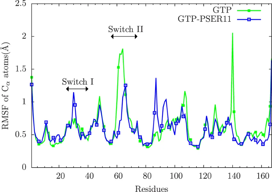
This plot shows that the RMSF(a measure to quantify fluctuations per amino acid in protein) patterns are different in the Rap protein in a Rap:Raf protein complex under 2 different conditions. Blue curve is the case where the protein Rap has a phosphorylated SER11. Green curve has no phosphorylation. You can see that the phosphorylation inhibits the motion of Rap protein at SWITCH-II region(57-74 residues). Ref:Phosphorylation promotes binding affinity of Rap-Raf complex by allosteric modulation of switch loop dynamics. License:CC Ver 4. Author's own work.

In this article, let us see how fluctuations and conformational changes of proteins in molecular dynamics(MD) simulations are quantified. Usually we quantify these using measures called:

RMSD (Root Mean Squared Deviation)
RMSF (Root Mean Squared Fluctuation)
PCA (Principal Component Analysis)
etc

A GIF movie illustrating fluctuations in a MD simulation trajectory of a Ubiquitin molecule. Only carbon alpha atoms of each amino acid is considered in this trajectory. The trajectory is 25ns long. Bluish regions at the tail are highly fluctating, whitish regions are fluctuating in a medium fashion and redish regions are least fluctutating. This trajectory was created by nullifying the translational and rotational motions and fitted with the crystal structure.

Repository

https://github.com/dexterdev/STEEMIT/tree/master/FLUCTUATIONS

What will I learn?

You will learn how to quantify the measures like RMSF, RMSD and PCA from biomolecular MD trajectories and deduce intuitions from the results.

Difficulty

Intermediate

System

The particular system which we are focusing on is a Ubiquitin simulation. The pdb file can be found here: 1UBQ. It has 76 aminoacids. We have mutated the 67th and 69th residue to SERINE amino acid. But this particular point is of no importance in this article, since our focus is on how to quantify fluctuations on an existing trajectory file. In case you are more interested in setting up MD simulations etc, you are advised to see my previous articles in this series. I have links to those articles at the bottom. I have simulated this ubiquitin structure in water with the mentioned mutations for 25ns. The force-field used was CHARMM27 version. The simulation was done using NAMD software. (For basics of MD and for setting up simulations in NAMD, see my previous articles. I am linking all required articles at the end in References.)

Softwares required:

VMD for molecular dynamics trajectory visualization and analysis scripting
MATLAB with matdcd plugin. matdcd is a popular DCD(our trajectory file format) reader/writer software which can be used with MATLAB.
(To be honest, for those who hate MATLAB and/or wanted a opensource software to work with there is MDTools for Python which is a python library to achieve the same. This is one among many other python options. Other tools include MDAnalysis and ProDy. But for this tutorial, I will stick to matdcd.)

Tutorial Contents

What is RMSD and RMSF?
What is PCA?
The relationship between PCA and RMSD
Extracting global motions of protein trajectory

What is RMSD and RMSF?

RMSD

RMSD(Root Mean Squared Deviation) is mathematically defined as:

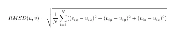
So let us break up the things and inspect. Let us think 'u' and 'v' as the two snapshots(x y z coordinates of two structures) of the same molecule at two different times in the same simulation. Say 'u' is the intitial structure of the molecule and 'v' be the strucutre after 10000 teps. 'N' is the number of atoms being considered. In the case of proteins, it is common to consider only carbon-alpha atoms only for each amino acid. So 'N' carbon alpha atoms are usually considered. RMSD gives a distance measure between conformations 'u' and 'v'. If you do this computation for every conformations in the MD trajectory keeping 'u' as a reference structure, you will end up with a data which will look like below:

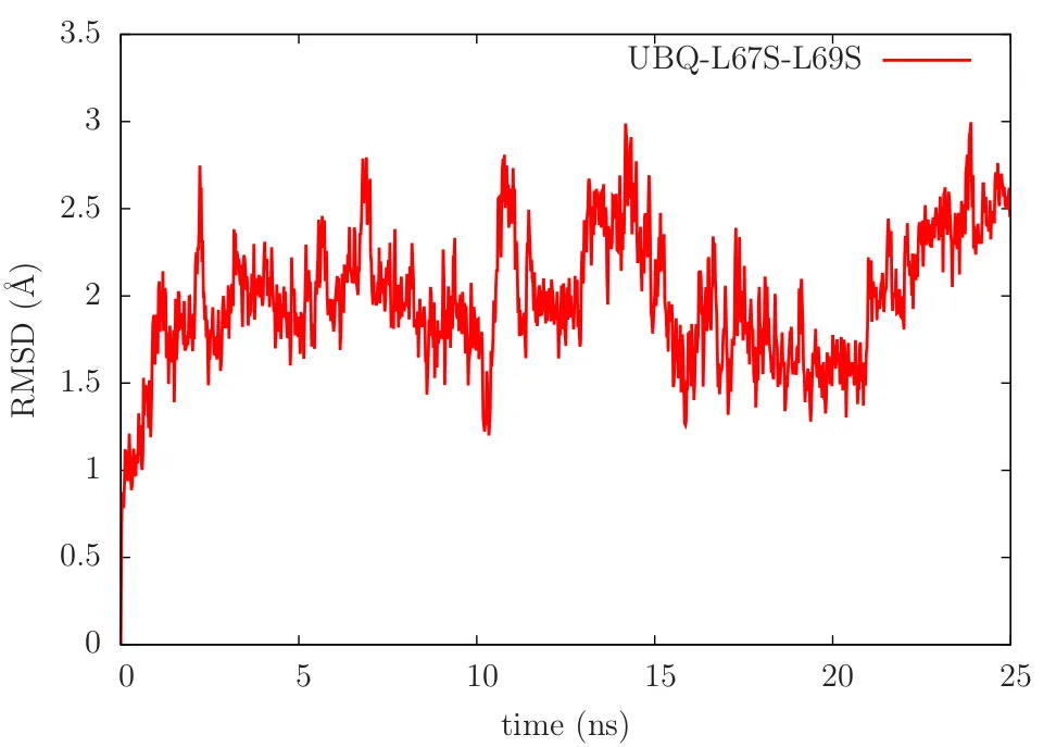
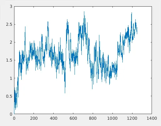
RMSD(u,v) plot of the ubiquitin system. Only alpha-carbon atoms considered.

RMSD(u,u)=0, which means that the RMSD measure between the same structures are zero. 'u' is the intitial strucutre here. Also, it is the reference structure. Once the MD simulation proceeds the structure changes. Which means 'v' keep on changing and once you stitch the whole data you get the RMSD plot as above. Two things to be noted:

If there is a sharp transition in the RMSD plot, it implies a conformational transition.
If the plot is more or less saturated(often accompanied by small fluctuations), it means that the protein is in a stable conformation. Butyou never know if it reached equilibrium or not. It is not uncommon that protein switiching conformation after staying in a different conformation for a long time period. This is a implication of the fact that the protein is sampling a free energy surface by visitng a lot of local minimas. Who knows where is the global minima? :P Oh I am deviating from the topic. Maybe more about those in a different article.

VMD tcl script to find RMSD between 2 structutes(assuming the structures have been fitted):

mol new ./ubq_L67S_L69S_CAfitted.psf.psf
mol addfile ./ubq_L67S_L69S_CAfitted.psf.dcd first 0 last -1 step 1 waitfor all
set sel1 [atomselect 0 "name CA" frame 0]
set sel2 [atomselect 0 "name CA" frame 10]
measure rmsd $sel1 $sel2
#finds rmsd of fitted structures between 1st and 11th frames

RMSF

RMSF(Root Mean square fluctutation) is related to RMSD. I will explain it in an intuitive way first before spitting out the equation. The first thing to note is that the reference structure in the case of RMSF is the time averaged strucutre from simulations instead of the intial strucutre as in RMSD. Say you need to find the RMSF corresponding to the last 5ns of MD data. You follow the steps as below:

Find the averaged strucutre(coordinates) for the last 5ns.
Do RMSD calculations separately for every N residue in the protein. But keep the reference coordinates('u') from the averaged structure.
Find the average of each RMSD calculations with respect to the frames(time axis).
Now you have an array of N numbers. This is your RMSF corresponding to the last 5ns.
The steps above make sense intutively. Computationally it may not be effective. Now to the equation:

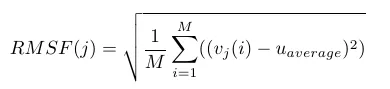
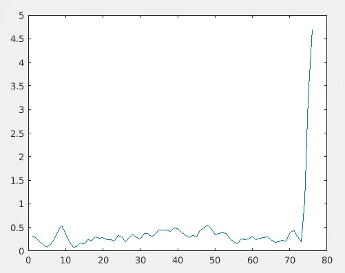
'M' is the number of frames considered from MD trajectory, RMSF(j) means the RMSF value corresponding to j-th residue. An example RMSF plot.

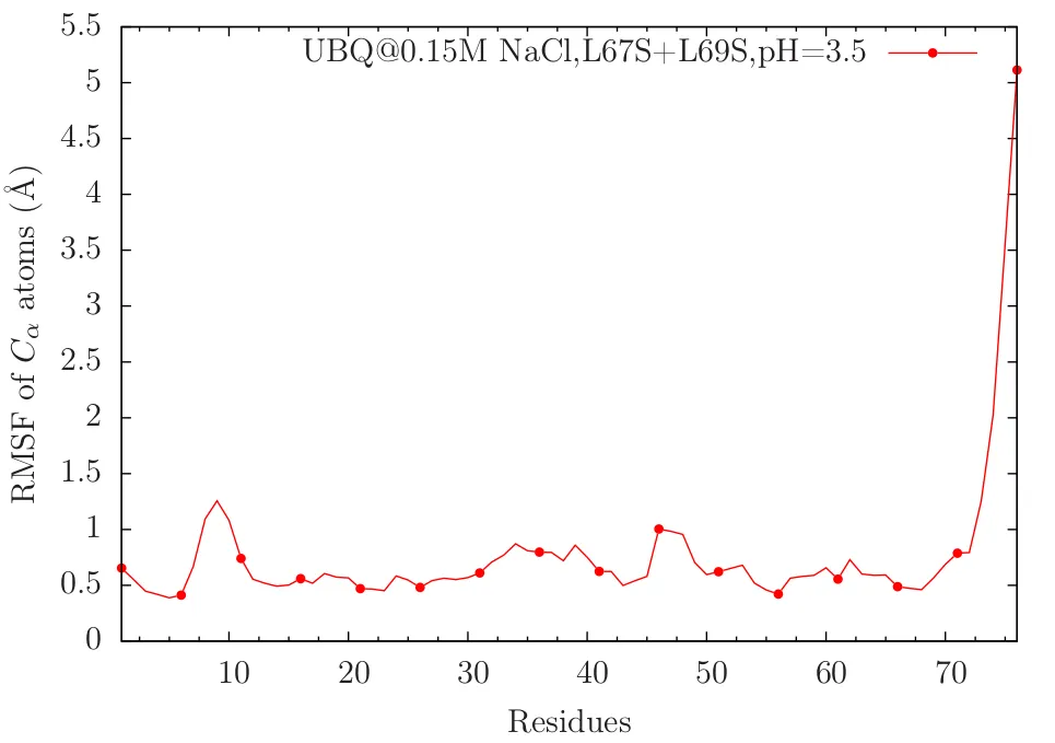
From the above plot, you can see that the C-terminal tail region of the protein is fluctuating very much. Residues around 10 and 48 are moderately fluctuating. One key point we learned are RMSD plot is w.r.t. time and RMSF plot is w.r.t. residues.

Fitting is important!! For all the RMSF and RMSD calculations, something which I didn't mentioned is this: You have to remove the translational and rotational motions from the protein to extract these measures. In VMD we can fit the trajectories to the intial structure(or whichever reference strucutre) using measure fit commands. A sample tcl script for vmd to write fitted carbon-alpha trajectory:

#load the raw dcd and psf files
mol new ./1UBQ_chain_pH3.5_L67S_L69S_waterbox_0.15molperL_NaCl.psf
mol addfile ./1UBQ_chain_pH3.5_L67S_L69S_waterbox_0.15molperL_NaCl.dcd first 0 last -1 step 1 waitfor all

#define the selection and reference strucutre, also find the total frame numbers
set sel  [atomselect 0 "name CA"]
set nf [molinfo 0 get numframes]
set f [expr $nf -1]
set ref_U1  [atomselect 0 "name CA" frame 0]

#fitting the trajectory for all frames in dcd file w.r.t. the initial frame
for {set i 1} {$i < $nf} {incr i} {
    set sel_U1 [atomselect 0 "name CA" frame $i]
    set M1 [measure fit $sel_U1 $ref_U1]
    $sel_U1 move $M1
}

#write the output dcd file and psf file
$ref_U1 writepsf ubq_L67S_L69S_CAfitted.psf
animate write dcd ubq_L67S_L69S_CAfitted.dcd beg 0 end $f waitfor all sel $sel

exit

What is PCA?

PCA a.k.a Principal Component Analysis is a very general statistical technique used for dimensionality reduction of higher dimensional data. To be honest, PCA will need a longer article by itself. But I suggest you to read this article if interested in learning it intuitively: https://sebastianraschka.com/Articles/2015_pca_in_3_steps.html
Here I will explain how to use PCA in MD context.

In the below figure, the second image can be considered as a dimensionally reduced one of first. Primarily the color information and minute details have been lost.

DIMENSIONALITY REUCTION 101: A cartoon depiction of dimensionality reduction. Credit for the above images goes to @atopy. I have adapted it. The second one can be considered as the dimensionally reduced @suesa.

When you talk about molecular dynamics trajectories, the dimension of data is Mx3N, where M is the number of frames of trajectory and N is the number of atoms(3N because of x y z position coordinates). The process of PCA can be summarised in the following steps:

Find the covariance matrix from the Mx3N coordiante matrix:

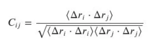
The delta-ri and delta-rj are the i-th and j-th atom displacements with respect to the corresponding reference structure atoms. The reference strucutre here is the intial strucutre.<.> represents the average values. The dimension of this Covariance matrix will be 3Nx3N.
Perform eigen value decomposition on the Covariance matrix. This will give you the eigen values corresponding covariance matrix. The highest eigen values and corresponding eigen vectors represent those data which contribute the global motions of the proteins.
Project the required eigen vectors to the data.

I will illustrate with an example. Let us start with the MATLAB code which uses the matdcd library.

clear, clc
xyz=readdcd('/home/devanandt/Documents/SIMULATION_TECHNIQUES_IN_BIOLOGY/NETWORK-ANALYSIS/ubq_L67S_L69S_CAfitted.dcd',1:76);
%readdcd from here: https://www.ks.uiuc.edu/Development/MDTools/matdcd/
[pc, score, latent, tsquare] = princomp(xyz);
score=score(:,1:3);%first 3 projected eigen vectors corresponding to the 3 highest eigen values
save PC_all_combined_ubq-fitted.dat score -ascii
pc1_percentage=latent(1)/sum(latent)%highest PC%
pc2_percentage=latent(2)/sum(latent)%second highest PC%

In the above code, princomp does the Covariance analysis and projection part. All we need to focus about is the latent(eigen values) and score(projected principal components). pc1_percentage and pc2_percentage are the percentage weights of the first 2 eigen values, which is around 35 and 19 respectively. Which means the first 2 Principal components have captured around 54% of the information in the 2 dimensions. So PCA is effectively finding the higher variance directions in the high dimensional data. The highest 2 directions are represented below:

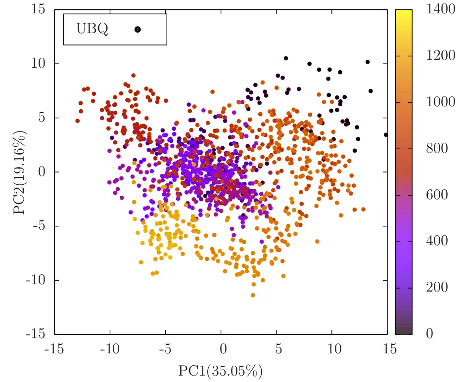
In the above plot, the colors encode time/frame axis. The black colored dots represent the intial structures and its evolution due to molecular dynamics equation. The yellowish dots represent the final states. There were 1250 frames(25ns) of DCD trajectory data.

The complete normalised eigen weights(PC percentages).

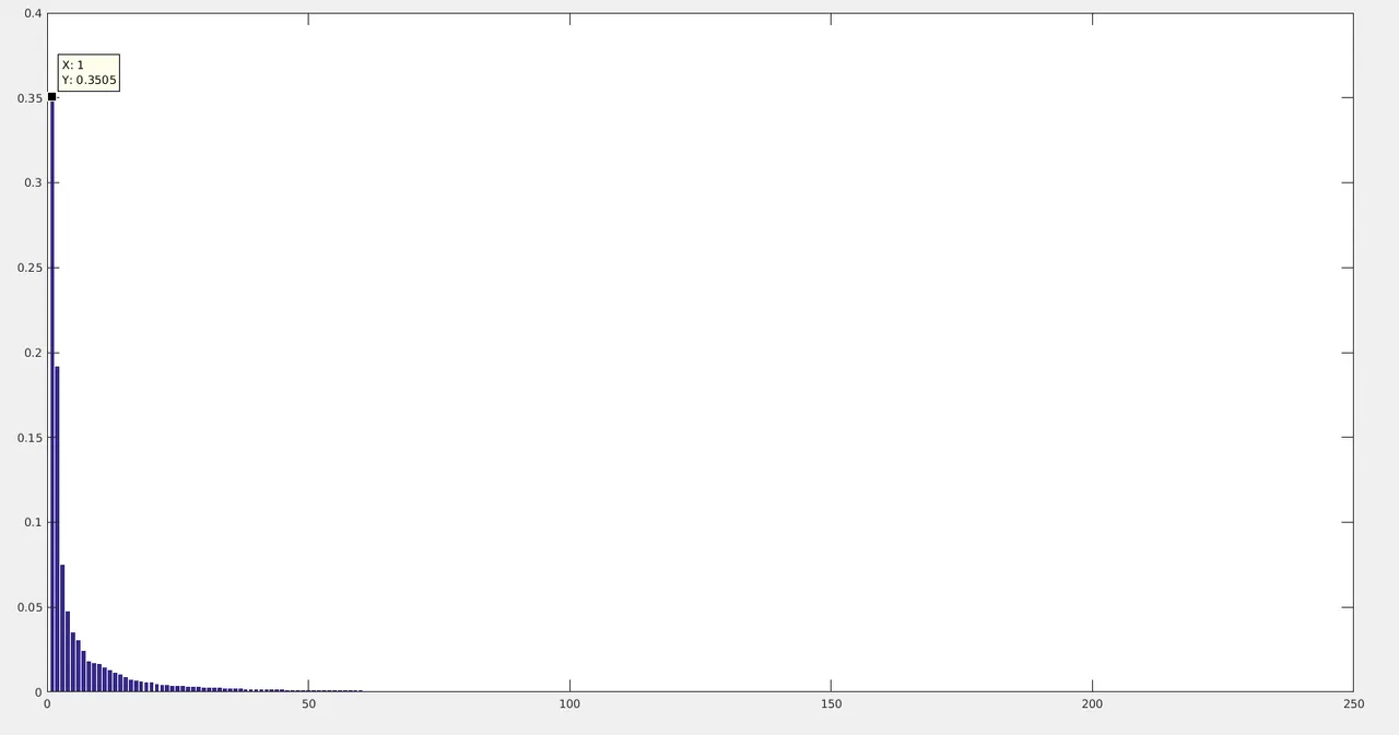
I would like to mention the main applications of PCA in MD data:

Is done to study the global motions in molecules (I will come to this later). i.e. To filter out the high frequency motions in the MD data.
To see the conformational space sampled by molecules

And there is a caveat people should know about when they use PCA: If the weight of eigen values captured by the first few vectors are less, it means that PCA will not be a meaningful tool in such particular cases! But most of the cases will have higher information content captured by the first few eigen vectors.

The relationship between PCA and RMSD

Yes, you can construct RMSD from PCA data. Let me prove it from a reverse-engineering process. The variable score(1250 rows x 3 columns) from the previous calculations:

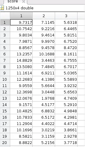
But we have only considered the first 2 PCs(columns) of this. Let us measure the euclidean distance measures of every row(considering first 2 columns only) w.r.t. the first row values(intial structure data).

for i=1:1250
d(i)=norm(score(i,1:2)-score(1,1:2));
end
plot(d)

This resembles RMSD plot, but the absolute values are very high comparing to original RMSD plots. The reason is that RMSD has a 1/sqrt(N) term. So you have to do that here too.

for i=1:1250
rmsd(i)=norm(score(i,1:2)-score(1,1:2))/sqrt(76);
end
plot(rmsd)

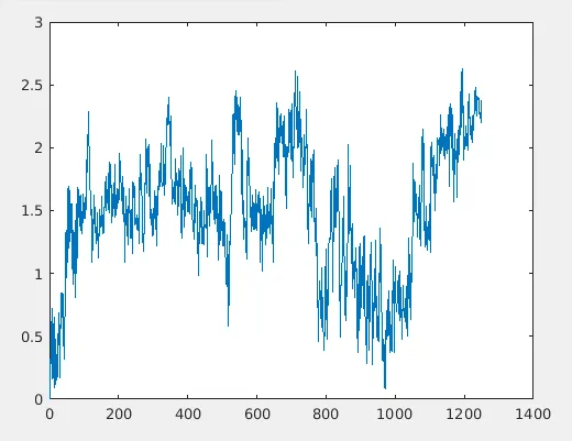
This is a 2D RMSD plot

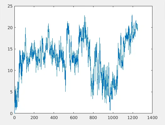
Let us increase the dimensions to 3 now.

for i=1:1250
rmsd(i)=norm(score(i,1:3)-score(1,1:3))/sqrt(76);
end
plot(rmsd)

3D RMSD plot
This is comparable with the original RMSD plot.

Original RMSD plot

Extracting global motions of protein trajectory

You can create a dimensionally reduced version of your trajectories by filtering out spurious motions. This will let you visualize the global motions(larger scale motions like opening and closing of structure etc). Let us create a 3D version of the original DCD.

% This reduces the dimension of ubiquitin CA dcd files to 3 D
clear,close,clc
xyz=readdcd('/home/devanandt/Documents/SIMULATION_TECHNIQUES_IN_BIOLOGY/NETWORK-ANALYSIS/ubq_L67S_L69S_CAfitted.dcd',1:76);
[U,S,V]=svd(xyz);%Eigen Value decomposition
xyz_r= U(:,[1:3])*S([1:3],[1:3])*V(:,[1:3])';
p=xyz_r;
x1=p(:,1:3:end);
y1=p(:,2:3:end);
z1=p(:,3:3:end);
rc = writedcd('3D_ubq.dcd',x1',y1',z1')

Compare this animation with the original gif at the top. This has less spurious small intensity vibrations.

Dimensionally reduced RMSF(considering only the first 3 strongest eigen values)

Original RMSF

Necessary Files

All necessary files are uploaded in Github.
https://github.com/dexterdev/STEEMIT/tree/master/FLUCTUATIONS

References

Research paper from which the first image is taken:

Phosphorylation promotes binding affinity of Rap-Raf complex by allosteric modulation of switch loop dynamics

My previous posts:

To learn about VMD and PDB file format, see here:

To learn about the concepts in All-atom molecular dynamics see articles below:

To setup and run simulations in NAMD software, see below:

Textbook references for learning theory of Molecular Dynamics:

"Statistical Mechanics: Theory and Molecular Simulations" by Mark E. Tuckerman
"Molecular Modelling: Principles and Applications" by Andrew R. Leach
"Computer Simulation of Liquids" by D. J. Tildesley and M.P. Allen

References specific to NAMD and VMD:

#steemSTEM

#steemSTEM is a very vibrant community on top of STEEM blockchain for Science, Technology, Engineering and Mathematics (STEM). If you wish to support steemstem visit the links below:

Have you voted for steemSTEM Witness?

Quick link for voting for the SteemSTEM Witness(@stem.witness)

Delegation links for @steemstem gives ROI of 65% of curation rewards

(quick delegation links: 50SP | 100SP | 500SP | 1000SP | 5000SP | 10000SP).

Also visit the steemstem app here: https://www.steemstem.io

All images without image sources are my creations :)

Follow me @dexterdev

 ____ _______  ______ _________ ____ ______    
/  _ /  __\  \//__ __/  __/  __/  _ /  __/ \ |\
| | \|  \  \  /  / \ |  \ |  \/| | \|  \ | | //
| |_/|  /_ /  \  | | |  /_|    | |_/|  /_| \// 
\____\____/__/\\ \_/ \____\_/\_\____\____\__/

credit: @mathowl

So bye bye friends. See you people with another interesting article. Till then STEEM ON!

Studying fluctuations in proteins from Molecular Dynamics trajectories