Image Processing - Visualisation
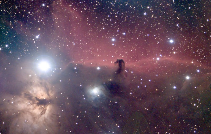
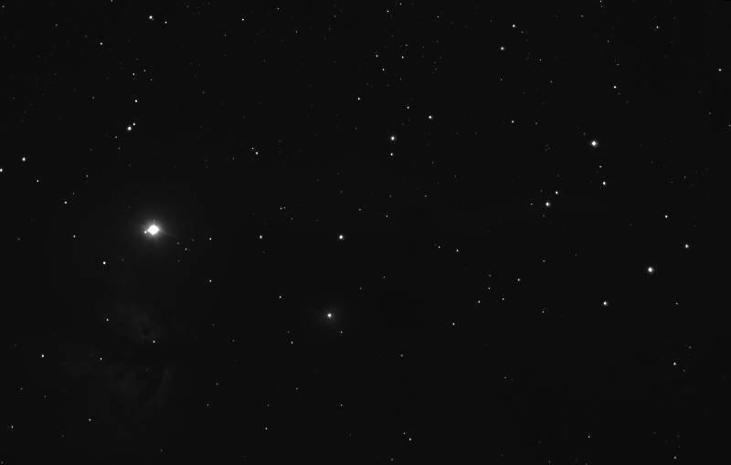
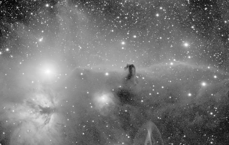
The Horsehead Nebula in Orion. Astronomical images have an enormous range of brightness, from the vanishing faint to bright stars, making it challenging to process to maximise the visible detail
In today's article, we look at the visualization of images, in particular adjusting brightness levels of an image to display all the visible detail. We look at the following topics:
- Image Stretch
- Histograms
- Non-Linear Stretch
- Histogram Stretching
Or the TLDR version : I've taken a photograph of the night sky and it's completely black and there is nothing there. How do I fix this!? Answer: Jump to section "Non-linear Stretch".
Image Stretch
Image Stretching is the process of adjusting the brightness and contrast of an image. Most people will be familiar with this when changing the brightness of a device screen. It is also analogous to turning the volume up or down on a speaker.
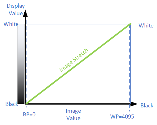
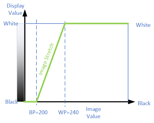
In a mathematical sense, the image pixel brightness values held in the computer's memory gets rescaled before being rendered on the screen. A simple linear image stretch can represent the green line in the following diagram. This line provides the mapping of image (in memory) values to displayed (on screen) values.
Stretch Diagram shows how the displayed pixel brightness maps to image pixel values
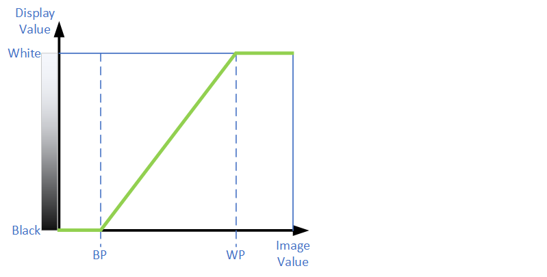
Here “BP” represents the black point or the pixel value which corresponds to black on the screen. Likewise, “WP” represents the white point or the pixel value which maps to white on the screen. Intermediate image pixels values between the black point and white point display as a grey level.
When the brightness is adjusted, the stretch diagram looks like the following. Note the black point, and white point is adjusted are shifted in unison as shown.
If contrast is adjusted, we see in the stretch diagram that Blackpoint and Whitepoint are moved closer or further apart. Contrast adjustment is demonstrated in the following diagram.

The histogram
A histogram of an image is a graph that displays the distribution of pixel brightness values in an image. It is a way of determining what proportion of an image is at a certain brightness. Many cameras have a histogram display in the viewfinder that enables correct estimation of exposure. Here is a typical image.
Daisy the Maltese "Bee-Dog"

Here is the histogram of that image.
Histogram of Daisy the Maltese "Bee-Dog"
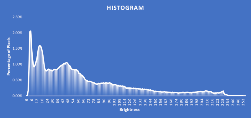
What does the histogram tell us in this image? First of all there about 253 (252 as well as the zero level) discrete brightness levels. This number of levels is typical of jpeg files which have brightness levels represented by 8-bit numbers that can represent a number from 0 to 255. However, what is significant is that most image has brightness values below above 70, judging by the peak in the histogram there. With no image, stretch applied this means that image is primarily dark, as 0 corresponds to black and 255 to white.
However, one other point to note is although the image is on the dark side, the histogram also tells us there are still significant numbers of brighter pixels from 70-228.
Histogram - Astronomical Images
Astronomical images tend to have very different histogram profiles when compared to daylight images. Let's look at the title image, converted to a 12-bit greyscale image (to simplify things). Here the image is stretched so the black point is at 0 and the white point is at 4095, which shows the entire brightness range of the image. It is almost entirely black apart from a handful of stars.
12-bit B/W converted version of title image. Without any image stretch the image looks almost completely black
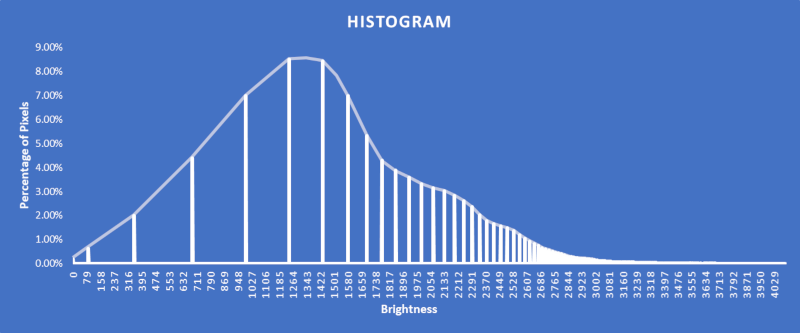
Looking at the histogram reveals that almost all the image pixels lay in a very narrow range of brightness values between 205 to 235. On the screen represents a very dark grey, almost black value which mean's the most of the image is black.
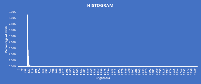
In the above image the stretch applied is blackpoint=0 and whitepoint=4095, represented as follows:
Since most of the pixel brightness values are between 205 and 235, let's choose a black point just under and a white point just over. A blackpoint=200 and whitepoint=240 is selected, so the stretch diagram looks like this:
The resultant displayed image looks like this. Quite an improvement and pretty much unrecognisable from the original image!
Above image displayed with an image stretch with blackpoint=200 and whitepoint=240. Considerable detail is now visible and it is amazing to think this is the same image. However, the brightest parts of the image are now over-exposed
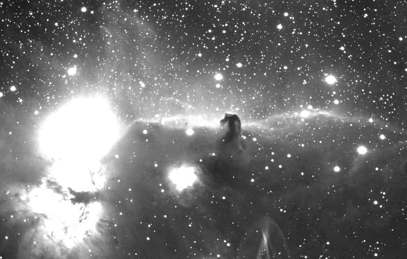
What we have discovered is most the image detail is locked up in this very narrow part of the histogram. The image looks a lot better, but unfortunately, some of the areas are "blown out and overexposed". This flaw is addressable, and this is what we shall look at now.
Non-linear Stretch
With a non-linear image stretch, we use a curve instead of a straight-line to map the image pixel brightness to the displayed pixel brightness. In this case, we shall use a logarithm function to generate the curve with the black point set to 190 and the white point to 4095.
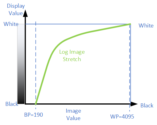
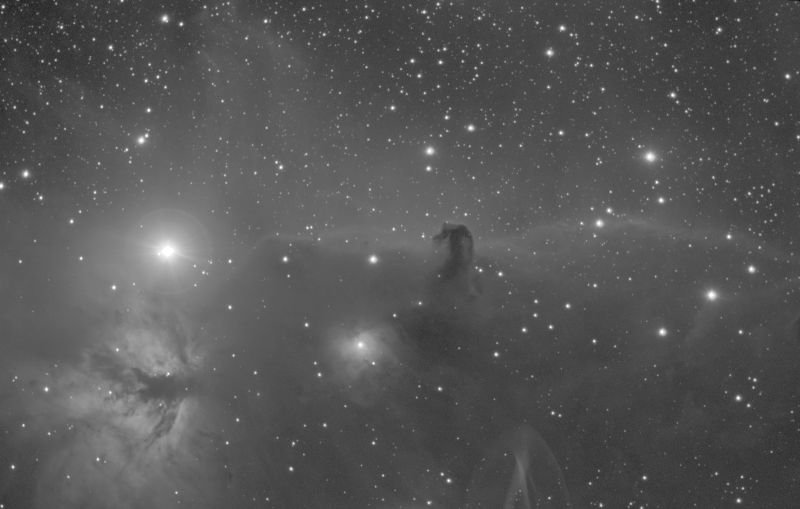
The resultant image is as follows. Notice that not only are the fainter areas displayed, but the highlights are also nicely visible. When you look at the curve above, notice that near the black point the green line is very steep which emulates the high contrast of the previous image, but the curve tapers off to prevent brighter parts from becoming too white. Human vision also has a logarithmic response which is why the image appears more natural.
A logarithm stretch with blackpoint=200 and whitepoint=4095. Not only is considerable detail in the fainter areas visible, but the brightest portions of the image are preserved
Note there are many other curves that can be used in place of logarithms like power functions (gamma) and many others.
Histogram Stretching methods
Another approach for preserving bright and dark detail is to use the image's histogram itself to rescale and stretch the pixel values. Many astronomical processing packages have this capability, and the easiest way to see the action is to look at the result, as well as the output histogram. The following image has been stretched, so it's histogram stretching with a target shape being Gaussian bell shape.
A Histogram stretch has been used with a target profile of a Gaussian peak. Compare this with some of the previous images
Here is the resulting histogram, compare this with the original narrow peak histogram from above.
Conclusions
This article was an introduction to image visualization for Astronomical imaging demonstrating the power of logarithm and Histogram stretching. In the next and final part, I shall complete the series by doing a review of suitable software for astronomical imaging, a lot of which is free.
Please note all images are the authors (unless otherwise noted)