최근 개인 신상이 변할 만한 일들이 생겨서 정말 ... 푹 쉬어버렸습니다.
2년동안 연구한 내용들이 아쉬워서 나름 정리를 해보려던 것이었는데, 정리가 늦어지고 말았습니다.
일단 쉬면서 정리한 내용들로 빠르게 마무리를 짓고 다른 내용으로 넘어가 보도록 하겠습니다.
지난번 글에서 글로만 정리하고 있었는데, 그림도 첨가 하면서 작성하도록 하겠습니다.
영상의 출처는 대부분 제가 추출했습니다. 그 코드는 LUNA16의 ipython 코드를 기초로 제가 수정한 코드를 사용합니다.
따로 출처가 있는 경우는 그 출처를 밝히도록 하겠습니다.
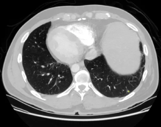
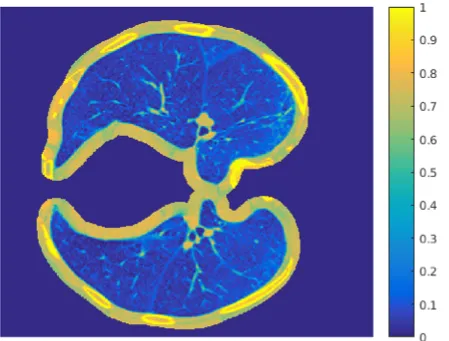
[Sample CT slide in LUNA16 challenge dataset]
너무 작아서 보기가 힘든데, 작은 노란색 + 표시가 있는 부분이 결절의 위치이다.
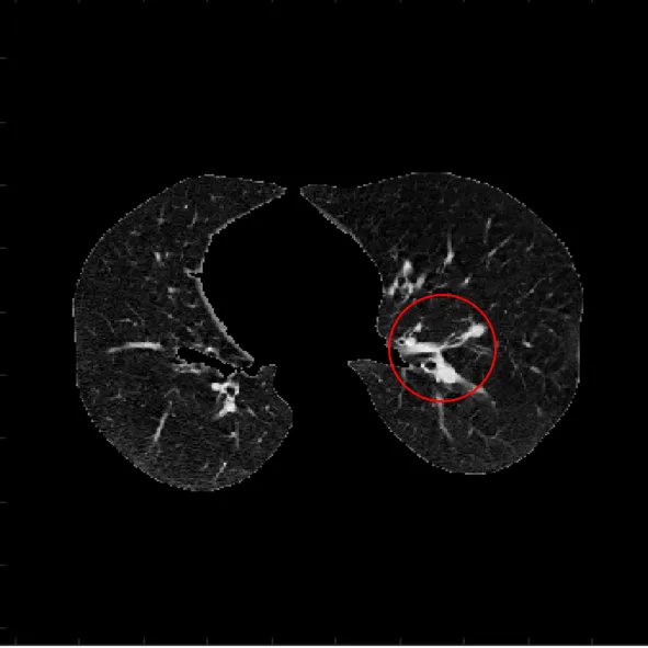
폐결절을 따로 확대해서 확인해 보면 아래와 같다.
오늘은 이 결절을 추출하는 단계까지 작성하겠다.
전 글에서 다른 연구들을 소개하려 했는데, 바로 넘어가는 것보다 그 부분을 이해하기 위한
기본 내용들도 중요하다 생각이 들어서 그부분을 먼저 정리 하고 넘어가겠다.
Preprocessing of pulmonary nodule extraction
폐결절 추출의 전처리 단계는 크게는 3단계로 이루어져있다.
- Hounsfield Unit (HU) Normalization
- Lung area segmentation
- Nodule detection
여기서 기존의 영상처리를 사용하는 시스템에서는 Lung area segmentation 에 대한 이슈가 있었는데, 최근의 Deep learning 을 통한 방법에서는 언급되지 않는다.
이 부분에 대해서는 나중에 Lung area 에서 그림과 함께 얘기 하도록 하겠다.
1. Hounsfield Unit Normalization
CT 영상은 방사선 (x-ray)가 인체를 투과하며 그 고유 물질에 따라 감쇠되는 정도가 다름을 이용하는 방식이다.
즉, 그 물질에 따라 다른 범위의 값을 갖는다. 이는 위키피디아에 매우 감사하게도 잘 정리되어있다.
[Wiki: Hounsfield Unit]https://en.wikipedia.org/wiki/Hounsfield_scale
LUNA16 의 tutorial 에서 사용하는 HU 값의 범위는 [-1000, 400]을 사용한다.
위키피디아의 Value in parts of the body 섹션의 표를 확인해 보면
이 범위의 HU값은 soft tissue를 포함해 많은 부분을 포함하는 값이라는 것을 확인 할 수 있다.
이처럼, 일정 범위의 HU 값을 [0, 1] 로 정규화(Normalization)하는 것은 특정 부분 만을 실험에 사용하기 위함이다.
먼저 영상을 불러 오기 위해 나는 Simple ITK를 사용해서 영상을 불러왔다.
import numpy as np
import SimpleITK as sitk

def load_itk_image(filename):
    itkimage = sitk.ReadImage(filename)
    numpyImage = sitk.GetArrayFromImage(itkimage) # z, y, x axis load
    numpyOrigin = np.array(list(reversed(itkimage.GetOrigin())))
    numpySpacing = np.array(list(reversed(itkimage.GetSpacing())))

    return numpyImage, numpyOrigin, numpySpacing
이때, 불러온 영상의 100번째 슬라이드를 출력한게 아래 그림이다.
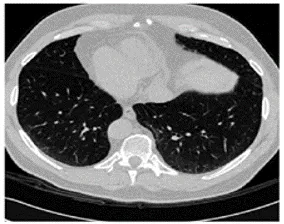
주의 할 점은 CT scan을 불러 올 때의 Array 순서에 따라 slide 의 방향이 바뀐다는 점이다.
내가 load 한 이미지를 확인했을 때는 array 가 [z, y, x] axis의 순서로 load 되었다.
Origin 과 Spacing 은 CT scan 의 해상도를 계산하기 위해 주어지는 정보이다.
우리에게 주어지는 폐결절의 정보인 지름(diameter)정보는 mm 단위로 주어지는데,
이 mm 단위를 pixel 단위로 변경하기 위해 사용되는 정보이다.
def normalizePlanes(npzarray):
    maxHU = 400.
    minHU = -1000.
    npzarray = (npzarray - minHU) / (maxHU - minHU)
    npzarray[ npzarray > 1 ] = 1.
    npzarray[ npzarray < 0 ] = 0.
    return npzarray

def chg_VoxelCoord(lists, str, origin, spacing):
    cand_list = []
    labels = []
    # if len(lists) > 2000:
    for list in lists:
        if list[0] in str:
            worldCoord =np.asarray([float(list[3]),float(list[2]),float(list[1])])
            voxelCoord = worldToVoxelCoord(worldCoord, origin, spacing)
            if list[4] is '1':
                augs, aug_labels = aug_candidate(voxelCoord)
                cand_list.append(voxelCoord)
                labels.append(int(list[4]))
                for aug in augs:
                    cand_list.append(aug)
                al_vec = np.ones((int(aug_labels),1))
                for aug_lbl in al_vec:
                    labels.append(int(aug_lbl))
            else:
                cand_list.append(voxelCoord)
                labels.append(int(list[4]))
    return cand_list, labels
numpy array 형식으로 load 한 데이터를 정규화 한 것이 npzarray 이다.
현실의 mm 단위를 pixel 단위로 변경하는 함수가 chg_VoxelCoord 이다.
이 함수를 통해 LUNA16에서 주어진 결절의 중심 좌표를 pixel 단위 좌표로 변경한다.
이제 normalized 이미지와 pixel 단위로 변환된 결절의 중심 위치를 얻었으니, patch 를 추출하기만 하면 되는 것이다.
2. Lung area segmentation
우선, 앞서 보여준 CT 영상에서 Lung area 를 추출하기 위한 방법으로 많이 사용되는 것이 앞서 언급한 HU 값을 이용하는 것이다.
HU 값의 Lung 범위의 중간점을 thresholding 하면 간단하게 Lung segmentation 영상을 확인 할 수 있다.
아래는 그 함수와 실행 결과 영상이다.
def make_lungmask(img, display=False):
    """
    # Standardize the pixel value by subtracting the mean and dividing by the standard deviation
    # Identify the proper threshold by creating 2 KMeans clusters comparing centered on soft tissue/bone vs lung/air.
    # Using Erosion and Dilation which has the net effect of removing tiny features like pulmonary vessels or noise
    # Identify each distinct region as separate image labels (think the magic wand in Photoshop)
    # Using bounding boxes for each image label to identify which ones represent lung and which ones represent "every thing else"
    # Create the masks for lung fields.
    # Apply mask onto the original image to erase voxels outside of the lung fields.
    """
    row_size = img.shape[0]
    col_size = img.shape[1]

    mean = np.mean(img)
    std = np.std(img)
    img = img - mean
    img = img / std
    # Find the average pixel value near the lungs
    # to renormalize washed out images
    middle = img[int(col_size / 5):int(col_size / 5 * 4), int(row_size / 5):int(row_size / 5 * 4)]
    mean = np.mean(middle)
    max = np.max(img)
    min = np.min(img)
    # To improve threshold finding, I'm moving the
    # underflow and overflow on the pixel spectrum
    img[img == max] = mean
    img[img == min] = mean

    # Using Kmeans to separate foreground (soft tissue / bone) and background (lung/air)
    kmeans = KMeans(n_clusters=2).fit(np.reshape(middle, [np.prod(middle.shape), 1]))
    centers = sorted(kmeans.cluster_centers_.flatten())
    threshold = np.mean(centers)
    thresh_img = np.where(img < threshold, 1.0, 0.0)  # threshold the image

    # First erode away the finer elements, then dilate to include some of the pixels surrounding the lung.
    # We don't want to accidentally clip the lung.

    eroded = morphology.erosion(thresh_img, np.ones([3, 3]))
    dilation = morphology.dilation(eroded, np.ones([8, 8]))

    labels = measure.label(dilation)  # Different labels are displayed in different colors
    label_vals = np.unique(labels)
    regions = measure.regionprops(labels)
    good_labels = []
    for prop in regions:
        B = prop.bbox
        if B[2] - B[0] < row_size / 10 * 9 and B[3] - B[1] < col_size / 10 * 9 and B[0] > row_size / 5 and B[
            2] < col_size / 5 * 4:
            good_labels.append(prop.label)
    mask = np.ndarray([row_size, col_size], dtype=np.int8)
    mask[:] = 0

    #
    #  After just the lungs are left, we do another large dilation
    #  in order to fill in and out the lung mask
    #
    for N in good_labels:
        mask = mask + np.where(labels == N, 1, 0)
    mask = morphology.dilation(mask, np.ones([10, 10]))  # one last dilation

    if display:
        fig, ax = plt.subplots(3, 2, figsize=[12, 12])
        ax[0, 0].set_title("Original")
        ax[0, 0].imshow(img, cmap='gray')
        ax[0, 0].axis('off')
        ax[0, 1].set_title("Threshold")
        ax[0, 1].imshow(thresh_img, cmap='gray')
        ax[0, 1].axis('off')
        ax[1, 0].set_title("After Erosion and Dilation")
        ax[1, 0].imshow(dilation, cmap='gray')
        ax[1, 0].axis('off')
        ax[1, 1].set_title("Color Labels")
        ax[1, 1].imshow(labels)
        ax[1, 1].axis('off')
        ax[2, 0].set_title("Final Mask")
        ax[2, 0].imshow(mask, cmap='gray')
        ax[2, 0].axis('off')
        ax[2, 1].set_title("Apply Mask on Original")
        ax[2, 1].imshow(mask * img, cmap='gray')
        ax[2, 1].axis('off')

        plt.show()
        plt.savefig('t.png')
    return mask * img
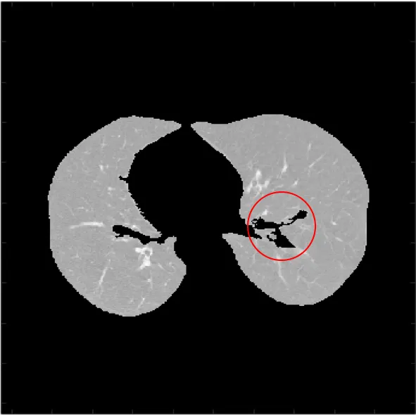
thresholding 의 결과 영상에서 빨간 원 안의 부분이 바로 맨처음에 언급한 issue 부분이다.
HU 을 기준으로 thresholding 을 하게 되면 기관지, 심장, 혈관등에 의해 일정 영역을 채울 수 없게 된다.
심장등이 위치한 아에 다른 영역이면 관련이 없지만, 종종 결절이 폐 가장자리에 발생하게 되면 body 영역과 유사한 HU 값 때문에 문제가 생기게 된다.
이런 문제를 해결하기위해 다양한 방법이 도입되었는데, 가장 대표적인 방법이 Lung area 를 조금 넓히는 방법이다.
또는 아래 처럼 LoG 필터를 사용하는 방법도 있는데, 이 부분은 MATLAB 으로 했는데 코드가 정리가 안되있어서 공개하진 않는다.
 [Rolling Ball]
 [LoG filter]
이런 부분은 영상처리에서 이슈가 되었지만, 딥러닝을 위한 patch 를 추출 할 때는 크게 신경쓰지 않아도 된다.
오히려 딥러닝에서는 HU normalization 의 의미가 좀더 중요해 진다.
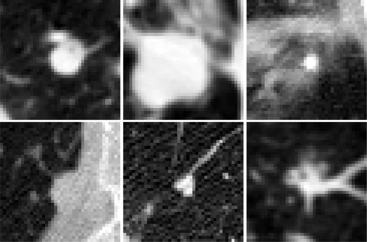
HU normalization issue
아래 그림은 각기 다른 HU 값으로 정규화한 동일 영역의 patch 이다.
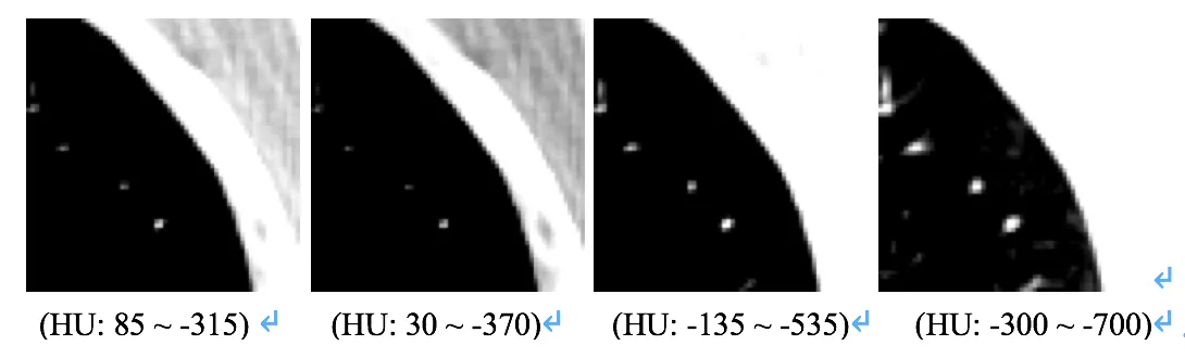
보이는 것과 같이 각 patch 들이 제공하는 정보가 각기 다름을 알 수 있다.
물론, 사용된 [-1000, 400] HU 값에는 위의 정보가 포함되어있다는 가정하에 실험이 진행되지만,
normalize 하는 HU 값의 변화에 따라 각 patch 가 가지는 정보의 의미가 변화한다는 것은 확인 할 수 있다.
본래 Convolutional Neural Network 의 실험을 위해서는 training set 과 validation set, test set 으로 구분하기 위한
Cross-validation 과정과 결절과 비결절의 불균형을 맞추기 위한 Augmentation 과정이 필요하지만,
이부분은 다른 글에서 더 잘 설명해주기 때문에 추가하지는 않았다.
오늘은 여기까지 ...